Getting started with admixr2 • admixr2

What is aggregate-data modelling?

admixr2 fits pharmacometric PK/PD models to summary-level data. For each clinical study you supply:

E — observed mean vector (one entry per observation time)
V — observed covariance matrix (or variance vector)
n — sample size
times — observation time points
ev — dosing event table

The estimator matches E and V against their model-predicted counterparts using a Monte Carlo approximation of the population distribution. This lets you apply established nlmixr2 models to aggregate statistics from publications or internal data summaries where individual records are unavailable.

Two backends are available:

Estimator	`est =`	Control function
Monte Carlo	`"admc"`	`admControl()`
Iterative Reweighting MC	`"adirmc"`	`adirmcControl()`

The examplomycin dataset

examplomycin ships with admixr2: 500 simulated subjects from a two-compartment PK model with first-order absorption (100 mg oral dose, sampled at 0.1, 0.25, 0.5, 1, 2, 3, 5, 8, and 12 h). True parameters: CL = 5 L/h, V1 = 10 L, V2 = 30 L, Q = 10 L/h, ka = 1 h⁻¹; IIV = 0.3 (SD on log scale) for all parameters; proportional error SD = 0.2.

library(admixr2)
library(rxode2)
library(nlmixr2)

data("examplomycin")
head(examplomycin[examplomycin$EVID == 0, c("ID", "TIME", "DV")], 9)
#>     ID  TIME    DV
#> 2  460  0.10 0.752
#> 3  460  0.25 1.932
#> 4  460  0.50 3.694
#> 5  460  1.00 3.479
#> 6  460  2.00 4.003
#> 7  460  3.00 3.825
#> 8  460  5.00 1.756
#> 9  460  8.00 1.155
#> 10 460 12.00 0.742

Computing aggregate statistics

Reshape individual records into a subjects × times matrix, then compute E and V:

obs   <- examplomycin[examplomycin$EVID == 0, ]
obs   <- obs[order(obs$ID, obs$TIME), ]
times <- sort(unique(obs$TIME))
ids   <- unique(obs$ID)
n     <- length(ids)                     # 500

dv_mat <- matrix(NA_real_, nrow = n, ncol = length(times))
for (i in seq_along(ids)) {
  sub         <- obs[obs$ID == ids[i], ]
  dv_mat[i, ] <- sub$DV[order(sub$TIME)]
}

E <- colMeans(dv_mat)
V <- cov(dv_mat)

round(E, 2)
#> [1] 0.97 1.94 2.79 3.02 2.26 1.65 1.06 0.75 0.51

V is the 9×9 sample covariance matrix. Its off-diagonal entries capture within-subject correlation across time; using the full matrix (method = "cov") typically tightens parameter estimates compared to the diagonal-only approximation (method = "var"). admixr2 auto-detects the method from the structure of V.

Model definition

Models use standard nlmixr2 syntax with mu-referenced log-scale parameters:

pk_model <- function() {
  ini({
    tcl     <- log(5)  ; label("Log clearance (L/hr)")
    tv1     <- log(10) ; label("Log central volume (L)")
    tv2     <- log(30) ; label("Log peripheral volume (L)")
    tq      <- log(10) ; label("Log inter-compartmental CL (L/hr)")
    tka     <- log(1)  ; label("Log absorption rate constant (1/hr)")
    prop.sd <- c(0, 0.2); label("Proportional residual error SD")
    eta.cl ~ 0.09
    eta.v1 ~ 0.09
    eta.v2 ~ 0.09
    eta.q  ~ 0.09
    eta.ka ~ 0.09
  })
  model({
    cl <- exp(tcl + eta.cl)
    v1 <- exp(tv1 + eta.v1)
    v2 <- exp(tv2 + eta.v2)
    q  <- exp(tq  + eta.q)
    ka <- exp(tka + eta.ka)
    d/dt(depot)      <- -ka * depot
    d/dt(central)    <- ka * depot - (cl/v1 + q/v1) * central + (q/v2) * peripheral
    d/dt(peripheral) <- (q/v1) * central - (q/v2) * peripheral
    cp <- central / v1
    cp ~ prop(prop.sd)
  })
}

Writing each parameter as exp(tcl + eta.cl) is called mu-referencing: the structural fixed effect and its random effect enter additively on the log scale. admixr2 exploits this pairing to compute analytical gradients via sensitivity equations. See the Advanced usage vignette for details, including how parameters without a random effect are handled.

Assembling the study specification

Bundle each study’s statistics into a named list:

study <- list(
  E     = E,
  V     = V,                       # full 9x9 covariance matrix
  n     = n,
  times = times,
  ev    = rxode2::et(amt = 100)    # single 100 mg oral dose
)

Fitting

Pass one or more named studies to admControl():

fit <- nlmixr2(
  pk_model, admData(), est = "admc",
  control = admControl(
    studies   = list(examplomycin = study),
    n_sim     = 5000L,
    cov_n_sim = 10000L,
    maxeval   = 300L,
    seed      = 1L
  )
)
#> [====|====|====|====|====|====|====|====|====|====] 0:00:07

Inspecting the fit

print(fit)
#> ── nlmixr² admc ──
#> 
#>           OBJF       AIC       BIC Log-likelihood
#> admc -3681.832 -3659.832 -3589.302       1840.916
#> 
#> ── Time (sec fit$time): ──
#> 
#>   optimize covariance elapsed
#> 1   44.579     10.456  55.035
#> 
#> ── Population Parameters (fit$parFixed or fit$parFixedDf): ──
#> 
#>                                   Parameter   Est.      SE   %RSE
#> tcl                    Log clearance (L/hr)  1.601 0.01636  1.022
#> tv1                  Log central volume (L)  2.315 0.08739  3.776
#> tv2               Log peripheral volume (L)  3.402 0.04014   1.18
#> tq        Log inter-compartmental CL (L/hr)  2.284 0.02133 0.9337
#> tka     Log absorption rate constant (1/hr) 0.0247 0.08218  332.6
#> prop.sd      Proportional residual error SD 0.1986               
#>         Back-transformed(95%CI) BSV(CV%) Shrink(SD)%
#> tcl         4.958 (4.802, 5.12)     32.8            
#> tv1        10.12 (8.529, 12.01)     33.8            
#> tv2        30.02 (27.75, 32.48)     32.0            
#> tq          9.82 (9.418, 10.24)     33.4            
#> tka       1.025 (0.8725, 1.204)     31.2            
#> prop.sd                  0.1986                     
#>  
#>   Covariance Type (fit$covMethod): r
#>   No correlations in between subject variability (BSV) matrix
#>   Full BSV covariance (fit$omega) or correlation (fit$omegaR; diagonals=SDs) 
#>   Distribution stats (mean/skewness/kurtosis/p-value) available in fit$shrink 
#>   Censoring (fit$censInformation): No censoring
#>   Minimization message (fit$message):  
#>     NLOPT_XTOL_REACHED: Optimization stopped because xtol_rel or xtol_abs (above) was reached.

Key entries in fit$env$admExtra:

fit$objective                    # -2 log-likelihood
#> [1] -3681.832
fit$env$admExtra$struct          # structural parameters (log scale)
#>        tcl        tv1        tv2         tq        tka 
#> 1.60108208 2.31477756 3.40198091 2.28442677 0.02470451
fit$env$admExtra$omega           # estimated Omega matrix
#>           [,1]      [,2]       [,3]      [,4]       [,5]
#> [1,] 0.1023461 0.0000000 0.00000000 0.0000000 0.00000000
#> [2,] 0.0000000 0.1079487 0.00000000 0.0000000 0.00000000
#> [3,] 0.0000000 0.0000000 0.09759912 0.0000000 0.00000000
#> [4,] 0.0000000 0.0000000 0.00000000 0.1057226 0.00000000
#> [5,] 0.0000000 0.0000000 0.00000000 0.0000000 0.09312475
fit$env$admExtra$sigma_var       # residual variance(s)
#>    prop.sd 
#> 0.03945189

logLik(fit)
#> 'log Lik.' 1840.916 (df=11)
AIC(fit)
#> [1] -3659.832

Diagnostic plots

plot() produces up to four panel types and returns them as a named list of ggplot2 objects:

plots <- plot(fit, which = c("mean", "nll"))

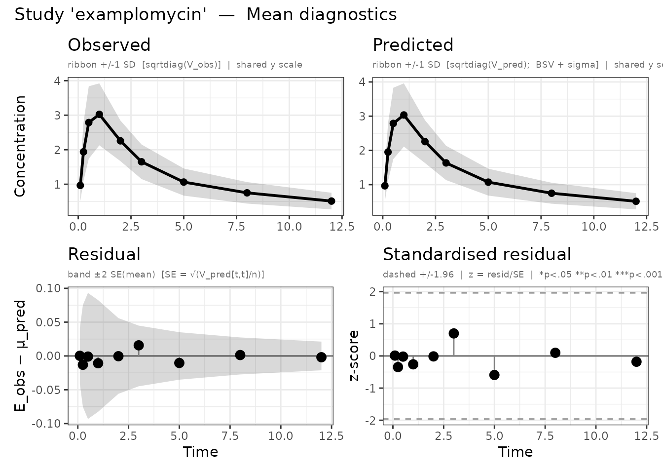
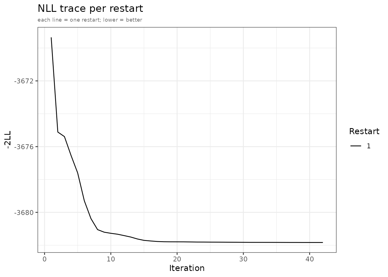
Left: observed vs predicted mean with residuals. Right: NLL convergence trace.

For a detailed walkthrough of all four panel types and customisation options, see vignette("diagnostic-plots", package = "admixr2").