Estimator comparison: adfo, admc, adgh and adirmc

Four estimators, one interface

All four estimators accept the same model and study specification and return the same admFit object. They share a common likelihood framework but differ in how they approximate the population mean and covariance of the predicted observations.

The shared integration problem

For each study the observed data are a mean vector $\bar{y}$ and a covariance matrix $S$ computed from $n$ subjects. Under a multivariate normal approximation the aggregate log-likelihood is

$$-2\ell = n \left[ \log |V_\text{pred}| + \operatorname{tr}(V_\text{pred}^{-1} S) + r^\top V_\text{pred}^{-1} r \right], \qquad r = \bar{y} - \mu_\text{pred}$$

where $\mu_\text{pred}$ and $V_\text{pred}$ are the model-predicted population mean and covariance of the observations. For a nonlinear model $f(\theta,\eta)$ these are integrals over the random-effects distribution $\eta \sim \mathcal{N}(0, \Omega)$:

$$\mu_\text{pred} = \mathbb{E}_\eta[f(\theta, \eta)], \qquad V_\text{pred} = \operatorname{Var}_\eta[f(\theta, \eta)] + \Sigma$$

These integrals have no closed form for nonlinear $f$. All four estimators minimise the same objective but take different approaches to evaluating them.

First-Order (FO): Taylor expansion at $\eta = 0$

adfo sidesteps the integral entirely by approximating $f(\theta, \eta)$ with its first-order Taylor expansion around $\eta = 0$:

$$f(\theta, \eta) \approx f(\theta, 0) + J\,\eta, \qquad J_{t,j} = \left.\frac{\partial f_t}{\partial \eta_j}\right|_{\eta=0}$$

Substituting into the population moments gives closed-form expressions:

$$\mu_\text{pred} = f(\theta, 0), \qquad V_\text{pred} = J\,\Omega\,J^\top + \Sigma$$

The Jacobian $J$ is obtained in a single rxSolve call via sensitivity equations that augment the ODE system with $\partial f / \partial \eta_j$ — no finite differences, no extra solves per eta. This makes adfo the fastest estimator: one rxSolve per NLL evaluation, fully deterministic.

When the approximation holds: the Taylor expansion is exact when $f$ is linear in $\eta$. For nonlinear models or large IIV the true population covariance exceeds $J\Omega J^\top$; FO underestimates $\Omega$ and bias grows with the degree of nonlinearity.

AIC note: adfo evaluates a linearised likelihood. Its objective is not on the same scale as admc or adirmc and must not be used for cross-estimator AIC comparisons.

Monte Carlo (MC): sample average over $\eta$

admc estimates the population integrals directly by drawing $N$ samples $\eta_i \sim \mathcal{N}(0, \Omega)$ and computing sample moments:

$$\mu_\text{pred} = \frac{1}{N} \sum_{i=1}^N f(\theta, \eta_i), \qquad V_\text{pred} = \frac{1}{N} \sum_{i=1}^N \bigl(f(\theta,\eta_i) - \mu_\text{pred}\bigr) \bigl(f(\theta,\eta_i) - \mu_\text{pred}\bigr)^\top + \Sigma$$

No approximation is made to $f$ itself — the estimator is asymptotically exact as $N \to \infty$. Sobol quasi-random sequences (default) reduce MC variance relative to plain normal draws, typically requiring 2–5× fewer samples for equivalent precision.

The key cost is that every NLL evaluation requires $N$ rxSolve calls — one per sample. The analytical gradient (sensitivity equations for mu-referenced parameters; common random numbers FD otherwise) adds no further solves, but the base cost per optimizer step remains $N \times$ (cost of one rxSolve).

Advantages:

• Asymptotically exact; AIC directly comparable across admc fits.
• Works well for standard 1–2 compartment PK models with moderate IIV.

Limitations:

• Each NLL evaluation requires $N$ rxSolve calls; slower than adfo.
• MC noise in the gradient can cause optimiser oscillation at low n_sim.

Iterative Reweighting MC (IRMC): proposals fixed, inner loop free

adirmc addresses the main bottleneck of admc — the need for $N$ new rxSolve calls at every optimizer step — by decoupling proposal generation from optimization.

At each outer phase, $N$ proposals $\eta_i$ are drawn once and held fixed for the entire inner optimization. Given fixed proposals, evaluating the NLL requires only matrix operations — no new rxSolve calls. The proposals are reweighted by their likelihood under the current $\Omega$ so that the inner objective remains a valid approximation as parameters move:

$$w_i \propto \frac{p(\eta_i \mid \Omega)}{q(\eta_i)}, \qquad \mu_\text{pred} = \sum_i w_i\, f(\theta, \eta_i), \qquad V_\text{pred} = \sum_i w_i\, \bigl(f(\theta,\eta_i) - \mu_\text{pred}\bigr) \bigl(\cdots\bigr)^\top + \Sigma$$

The inner optimizer therefore runs to convergence at negligible cost; proposals are refreshed only between phases. Box constraints on the parameters are progressively tightened across phases to guide global convergence.

This decoupling makes adirmc particularly well-suited to complex ODE models where each rxSolve is expensive: the total number of solves scales with the number of phases rather than the number of optimizer steps. It is also more robust to poor starting values because the inner optimisation is deterministic and does not depend on re-sampling.

Advantages:

• Far fewer rxSolve calls per optimizer step than admc — especially beneficial for complex ODE systems with expensive solves.
• Robust to poor starting values; deterministic inner loop.
• AIC directly comparable to admc.

Limitations:

• Heavier per-phase overhead than admc for simple, well-initialised problems with cheap ODE solves.

Gauss-Hermite (GH): deterministic quadrature over $\eta$

adgh evaluates the population integrals exactly (up to the accuracy of the quadrature rule) using a tensor-product Gauss-Hermite grid over $\eta \sim \mathcal{N}(0, \Omega)$. The nodes $\eta_q$ and weights $w_q$ are computed via the Golub-Welsch algorithm; $L\eta_q$ applies the Cholesky factor to map standard-normal nodes into the correlated $\eta$ space:

$$\mu_\text{pred} = \sum_{q=1}^Q w_q\, f(\theta, \eta_q), \qquad V_\text{pred} = \sum_{q=1}^Q w_q\, \bigl(f(\theta,\eta_q) - \mu_\text{pred}\bigr) \bigl(\cdots\bigr)^\top + \Sigma$$

With $m$ nodes per dimension and $n_\eta$ random effects the grid has $Q = m^{n_\eta}$ points. The objective is fully deterministic — no MC noise — so the gradient is clean and the Hessian well-conditioned.

Advantages:

• Noise-free objective — cleaner gradient than MC; reproducible across runs without fixing n_sim.
• AIC directly comparable to admc and adirmc (same likelihood scale).
• For models with $\leq 4$ etas, $Q$ is small (e.g. $5^4 = 625$) and adgh is substantially faster than admc at equivalent accuracy.
• Unbiased at any IIV magnitude (unlike FO); no approximation to $f$.

Limitations:

• Node count grows exponentially: $5^5 = 3125$, $5^6 = 15625$. For high-dimensional IIV consider admc or adirmc.
• No inner-loop cost saving for complex ODE systems (unlike adirmc); each NLL evaluation runs all $Q$ rxSolve calls.

Common setup

library(admixr2)
library(rxode2)
library(nlmixr2)
library(ggplot2)

data("examplomycin")
obs   <- examplomycin[examplomycin$EVID == 0, ]
obs   <- obs[order(obs$ID, obs$TIME), ]
times <- sort(unique(obs$TIME))
ids   <- unique(obs$ID)
n     <- length(ids)

dv_mat <- matrix(NA_real_, nrow = n, ncol = length(times))
for (i in seq_along(ids)) {
  sub         <- obs[obs$ID == ids[i], ]
  dv_mat[i, ] <- sub$DV[order(sub$TIME)]
}
E <- colMeans(dv_mat)
V <- cov.wt(dv_mat, method = "ML")$cov

pk_model <- function() {
  ini({
    tcl     <- log(5)  ; label("Log clearance (L/hr)")
    tv1     <- log(10) ; label("Log central volume (L)")
    tv2     <- log(30) ; label("Log peripheral volume (L)")
    tq      <- log(10) ; label("Log inter-compartmental CL (L/hr)")
    tka     <- log(1)  ; label("Log absorption rate constant (1/hr)")
    prop.sd <- c(0, 0.2); label("Proportional residual error SD")
    eta.cl ~ 0.09
    eta.v1 ~ 0.09
    eta.v2 ~ 0.09
    eta.q  ~ 0.09
    eta.ka ~ 0.09
  })
  model({
    cl <- exp(tcl + eta.cl)
    v1 <- exp(tv1 + eta.v1)
    v2 <- exp(tv2 + eta.v2)
    q  <- exp(tq  + eta.q)
    ka <- exp(tka + eta.ka)
    d/dt(depot)      <- -ka * depot
    d/dt(central)    <- ka * depot - (cl/v1 + q/v1) * central + (q/v2) * peripheral
    d/dt(peripheral) <- (q/v1) * central - (q/v2) * peripheral
    cp <- central / v1
    cp ~ prop(prop.sd)
  })
}

study <- list(E = E, V = V, n = n, times = times, ev = rxode2::et(amt = 100))

The model uses mu-referenced parameterisation (cl <- exp(tcl + eta.cl)), which enables analytical gradient computation via sensitivity equations in all four estimators. See the Advanced usage vignette for details.

Fitting with adfo

adfo is the fastest estimator and a natural starting point for model screening or obtaining initial estimates for MC refinement.

fit_fo <- nlmixr2(
  pk_model, admData(), est = "adfo",
  control = adfoControl(
    studies  = list(examplomycin = study),
    maxeval  = 500L,
    seed     = 1L
  )
)

Fitting with admc

fit_mc <- nlmixr2(
  pk_model, admData(), est = "admc",
  control = admControl(
    studies   = list(examplomycin = study),
    n_sim     = 5000L,
    cov_n_sim = 10000L,
    maxeval   = 300L,
    seed      = 1L
  )
)
#> [====|====|====|====|====|====|====|====|====|====] 0:00:07

Fitting with adirmc

adirmc is slower per evaluation but more robust to poor starting values and high-dimensional $\Omega$. The settings below are tuned for a fast vignette build; increase n_sim for production use.

fit_irmc <- nlmixr2(
  pk_model, admData(), est = "adirmc",
  control = adirmcControl(
    studies         = list(examplomycin = study),
    n_sim           = 2000L,
    phases          = c(2, 1, 0.5, 0.1),
    cov_n_sim       = 10000L,
    omega_expansion = 1.5,
    seed            = 1L
  )
)

Fitting with adgh

adgh is a drop-in alternative to admc for models with a modest number of etas. The five-eta model used here produces $5^5 = 3125$ nodes — at the upper end of practical use. For production fits consider n_nodes = 3 (243 nodes) as a fast starting point, increasing to 5 or 7 if IIV is large (SD > 0.4).

fit_gh <- nlmixr2(
  pk_model, admData(), est = "adgh",
  control = adghControl(
    studies  = list(examplomycin = study),
    n_nodes  = 5L,
    maxeval  = 300L,
    seed     = 1L
  )
)

Comparing parameter estimates

adfo and admc should recover values close to the true parameters (CL = 5, V1 = 10, V2 = 30, Q = 10, ka = 1; IIV variance = 0.09 for all; prop.sd = 0.2). For the examplomycin dataset IIV is moderate and the model is near-linear in $\eta$, so FO bias is small.

get_pars <- function(fit) {
  s  <- fit$env$admExtra$struct
  om <- diag(fit$env$admExtra$omega)
  sg <- sqrt(unlist(fit$env$admExtra$sigma_var))
  c(exp(s), om, sg)
}

tbl <- data.frame(
  Parameter = c(
    paste0("exp(", names(fit_fo$env$admExtra$struct), ")"),
    paste0("var(", fit_fo$env$admExtra$eta_col_names, ")"),
    "prop.sd"
  ),
  True = c(5, 10, 30, 10, 1, rep(0.09, 5), 0.2),
  adfo = round(get_pars(fit_fo), 4),
  admc = round(get_pars(fit_mc), 4)
)

knitr::kable(tbl, caption = "Parameter estimates vs true values")

Parameter estimates vs true values

Parameter	True	adfo	admc
exp(tcl)	5.00	4.9305	4.9583
exp(tv1)	10.00	7.5125	10.1172
exp(tv2)	30.00	31.7752	30.0312
exp(tq)	10.00	10.3718	9.8217
exp(tka)	1.00	0.8336	1.0245
var(eta.cl)	0.09	0.0972	0.1022
var(eta.v1)	0.09	0.1309	0.1080
var(eta.v2)	0.09	0.0728	0.0975
var(eta.q)	0.09	0.1015	0.1056
var(eta.ka)	0.09	0.0872	0.0928
prop.sd	0.20	0.1998	0.1984

Comparing objectives

admc and adirmc evaluate the same likelihood and their -2LL values are directly comparable. adfo evaluates a linearised likelihood — its objective is on a different scale and must not be compared with MC objectives or used for cross-estimator AIC:

cat(sprintf("adfo  -2LL = %.2f   AIC = %.2f\n", fit_fo$objective, AIC(fit_fo)))
#> adfo  -2LL = -3675.39   AIC = -3653.39
cat(sprintf("admc  -2LL = %.2f   AIC = %.2f\n", fit_mc$objective, AIC(fit_mc)))
#> admc  -2LL = -3690.84   AIC = -3668.84

Use AIC only within the same estimator for model selection.

NLL convergence traces

plots_fo <- plot(fit_fo, which = "nll")

adfo and admc NLL convergence traces.

plots_mc <- plot(fit_mc, which = "nll")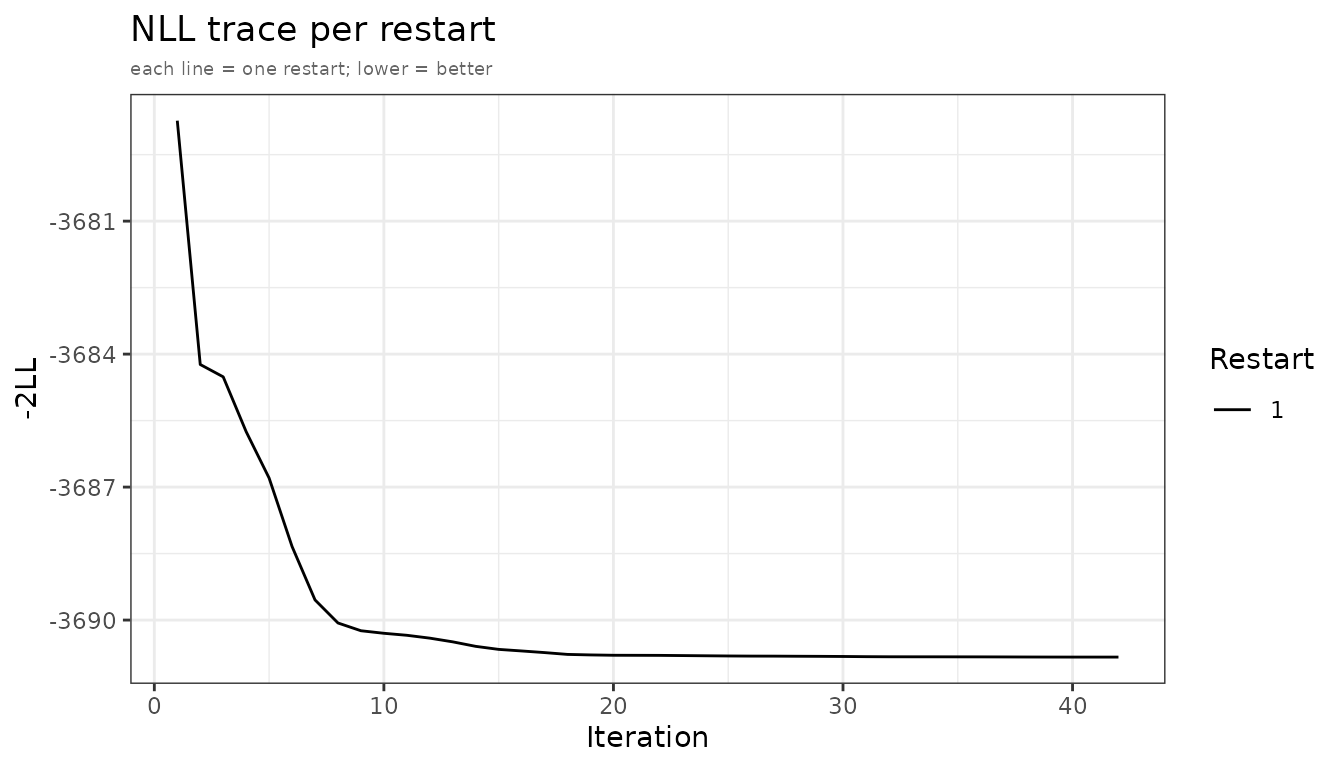

adfo and admc NLL convergence traces.

For adirmc, the NLL trace reflects outer phase iterations rather than individual LBFGS steps. Jumps between phases (as box constraints tighten) are normal and expected.

When to use each

Situation	Recommendation
Rapid model screening, many candidate models	adfo — fastest per evaluation
Initial estimates before MC/GH refinement	adfo then hand off to admc or adgh
Weak IIV (CV < 20 %) and near-linear model	adfo estimates reliable for inference
Standard 1–2 compartment PK, ≤ 4 etas	adgh — noise-free, faster than MC at equivalent accuracy
Standard 1–2 compartment PK, ≥ 5 etas or large IIV	admc with grad = "sens"
Initial exploration or poor starting values	admc with n_restarts >= 3
Complex ODE system with expensive solves	adirmc — inner loop needs no new rxSolve calls
High-dimensional Omega (≥ 5 etas)	adirmc — inner loop scales with phases not steps
Non-Gaussian or bounded IIV	adirmc with omega_expansion > 1
Optimal design / design evaluation (matched moments)	adgh with datagenControl(method = "gh")
Need exact likelihood for AIC comparison across models	admc, adgh, or adirmc (not adfo)
Maximum reproducibility, no MC noise	adfo or adgh (both deterministic)

Control objects at a glance

# adfo key arguments (fastest; linearised likelihood)
adfoControl(
  studies    = list(...),
  grad       = "none",      # "none" (BOBYQA), "analytical", "fd", "cfd"
  maxeval    = 500L,
  n_restarts = 1L,
  covMethod  = "r",         # SEs for struct+sigma only; omega SEs are not computed
  seed       = 1L
)

# admc key arguments
admControl(
  studies    = list(...),
  n_sim      = 5000L,       # MC sample count
  grad       = "sens",      # gradient mode: "sens", "fd", "cfd", "none"
  n_restarts = 1L,          # number of optimizer restarts
  workers    = 1L,          # parallel workers for restarts
  covMethod  = "r",         # SEs for struct+sigma only; omega SEs are not computed
  seed       = 1L
)

# adgh key arguments (noise-free quadrature; same likelihood scale as admc)
adghControl(
  studies    = list(...),
  n_nodes    = 5L,          # nodes per eta dimension; total = n_nodes^n_eta
  grad       = "analytical",# gradient mode: "analytical", "fd", "cfd", "none"
  n_restarts = 1L,
  workers    = 1L,
  covMethod  = "r",         # SEs for struct+sigma only
  seed       = 1L
)

# adirmc key arguments
adirmcControl(
  studies         = list(...),
  n_sim           = 5000L,
  phases          = c(2, 1, 0.5, 0.1),   # box constraint half-widths per phase
  omega_expansion = 1.5,                   # inflate proposal Omega
  grad            = "analytical",          # "analytical", "none", "fd"
  kappa_method    = "exact",               # "exact", "linearized", "linearized_gh"
  seed            = 1L
)