Why multiple studies?
Passing several studies to admControl() fits the model
to all of them simultaneously, minimising the sum of per-study NLLs
under a shared set of population parameters. This is the core use case
for aggregate-data modelling: you have summary statistics from multiple
trials (which may differ in dose, sample size, or observation schedule)
and want a single population model consistent with all of them.
Splitting examplomycin into two cohorts
We partition the 500 examplomycin subjects into two cohorts of 250 and compute separate aggregate statistics for each:
library(admixr2)
library(rxode2)
library(nlmixr2)
library(ggplot2)

data("examplomycin")
obs   <- examplomycin[examplomycin$EVID == 0, ]
obs   <- obs[order(obs$ID, obs$TIME), ]
times <- sort(unique(obs$TIME))
ids   <- unique(obs$ID)

dv_mat <- matrix(NA_real_, nrow = length(ids), ncol = length(times))
for (i in seq_along(ids)) {
  sub         <- obs[obs$ID == ids[i], ]
  dv_mat[i, ] <- sub$DV[order(sub$TIME)]
}

# Alternate subjects into two equal cohorts
idx1 <- seq(1, length(ids), by = 2)   # rows 1, 3, 5, ... → cohort 1
idx2 <- seq(2, length(ids), by = 2)   # rows 2, 4, 6, ... → cohort 2

E1 <- colMeans(dv_mat[idx1, ]); V1 <- cov.wt(dv_mat[idx1, ], method = "ML")$cov; n1 <- length(idx1)
E2 <- colMeans(dv_mat[idx2, ]); V2 <- cov.wt(dv_mat[idx2, ], method = "ML")$cov; n2 <- length(idx2)
Comparing observed profiles across cohorts
Before fitting, visualise the raw summary statistics to confirm the two cohorts are comparable (both drawn from the same population here):
df_obs <- rbind(
  data.frame(cohort = "Cohort 1", time = times,
             mean = E1,
             lo   = E1 - sqrt(diag(V1)),
             hi   = E1 + sqrt(diag(V1))),
  data.frame(cohort = "Cohort 2", time = times,
             mean = E2,
             lo   = E2 - sqrt(diag(V2)),
             hi   = E2 + sqrt(diag(V2)))
)

ggplot(df_obs, aes(x = time, y = mean, colour = cohort, fill = cohort)) +
  geom_ribbon(aes(ymin = lo, ymax = hi), alpha = 0.15, colour = NA) +
  geom_line(linewidth = 1) +
  geom_point(size = 2.5) +
  scale_x_log10(breaks = times, labels = times) +
  scale_colour_manual(values = c("Cohort 1" = "#0072B2", "Cohort 2" = "#D55E00")) +
  scale_fill_manual(  values = c("Cohort 1" = "#0072B2", "Cohort 2" = "#D55E00")) +
  labs(title    = "Observed mean ± 1 SD by cohort",
       x        = "Time (h, log scale)",
       y        = "Concentration",
       colour   = NULL, fill = NULL) +
  theme_bw()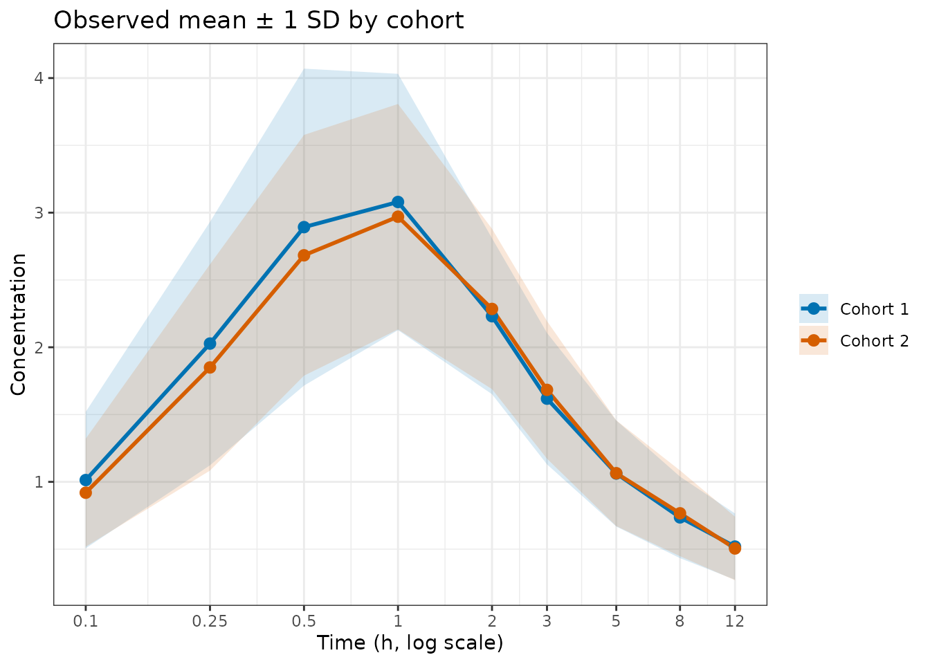
Observed mean ± 1 SD for each cohort on a log time axis.
Model definition
pk_model <- function() {
  ini({
    tcl     <- log(5)  ; label("Log clearance (L/hr)")
    tv1     <- log(10) ; label("Log central volume (L)")
    tv2     <- log(30) ; label("Log peripheral volume (L)")
    tq      <- log(10) ; label("Log inter-compartmental CL (L/hr)")
    tka     <- log(1)  ; label("Log absorption rate constant (1/hr)")
    prop.sd <- c(0, 0.2); label("Proportional residual error SD")
    eta.cl ~ 0.09
    eta.v1 ~ 0.09
    eta.v2 ~ 0.09
    eta.q  ~ 0.09
    eta.ka ~ 0.09
  })
  model({
    cl <- exp(tcl + eta.cl)
    v1 <- exp(tv1 + eta.v1)
    v2 <- exp(tv2 + eta.v2)
    q  <- exp(tq  + eta.q)
    ka <- exp(tka + eta.ka)
    d/dt(depot)      <- -ka * depot
    d/dt(central)    <- ka * depot - (cl/v1 + q/v1) * central + (q/v2) * peripheral
    d/dt(peripheral) <- (q/v1) * central - (q/v2) * peripheral
    cp <- central / v1
    cp ~ prop(prop.sd)
  })
}
Fitting with two studies
Pass both cohorts as a named list. Each entry may independently
specify times, ev, V,
n, and method:
fit_multi <- nlmixr2(
  pk_model, admData(), est = "admc",
  control = admControl(
    studies = list(
      cohort1 = list(E = E1, V = V1, n = n1,
                     times = times, ev = rxode2::et(amt = 100)),
      cohort2 = list(E = E2, V = V2, n = n2,
                     times = times, ev = rxode2::et(amt = 100))
    ),
    n_sim     = 5000L,
    cov_n_sim = 10000L,
    maxeval   = 300L,
    seed      = 1L
  )
)
#> [====|====|====|====|====|====|====|====|====|====] 0:00:07
#>
#> [====|====|====|====|====|====|====|====|====|====] 0:00:07

print(fit_multi)
#> ── nlmixr² admc ──
#>
#>           OBJF       AIC       BIC Log-likelihood
#> admc -3690.835 -3668.835 -3598.305       1845.418
#>
#> ── Time (sec fit_multi$time): ──
#>
#>   optimize covariance elapsed
#> 1    77.14     18.349  95.489
#>
#> ── Population Parameters (fit_multi$parFixed or fit_multi$parFixedDf): ──
#>
#>                                   Parameter    Est.      SE   %RSE
#> tcl                    Log clearance (L/hr)   1.601 0.01635  1.021
#> tv1                  Log central volume (L)   2.314 0.08719  3.768
#> tv2               Log peripheral volume (L)   3.402 0.04007  1.178
#> tq        Log inter-compartmental CL (L/hr)   2.285 0.02132 0.9332
#> tka     Log absorption rate constant (1/hr) 0.02423 0.08198  338.4
#> prop.sd      Proportional residual error SD  0.1984
#>         Back-transformed(95%CI) BSV(CV%) Shrink(SD)%
#> tcl         4.958 (4.802, 5.12)     32.8
#> tv1           10.12 (8.528, 12)     33.8
#> tv2        30.03 (27.76, 32.48)     32.0
#> tq          9.822 (9.42, 10.24)     33.4
#> tka       1.025 (0.8725, 1.203)     31.2
#> prop.sd                  0.1984
#>
#>   Covariance Type (fit_multi$covMethod): r
#>   No correlations in between subject variability (BSV) matrix
#>   Full BSV covariance (fit_multi$omega)
#>     or correlation (fit_multi$omegaR; diagonals=SDs)
#>   Distribution stats (mean/skewness/kurtosis/p-value) available in $shrink
#>   Censoring (fit_multi$censInformation): No censoring
#>   Minimization message (fit_multi$message):
#>     NLOPT_XTOL_REACHED: Optimization stopped because xtol_rel or xtol_abs (above) was reached.
Per-study diagnostic plots
plot() automatically produces separate panels for each
study. Panel names follow the pattern mean_<study>
and cov_<study>:
plots <- plot(fit_multi, which = "mean")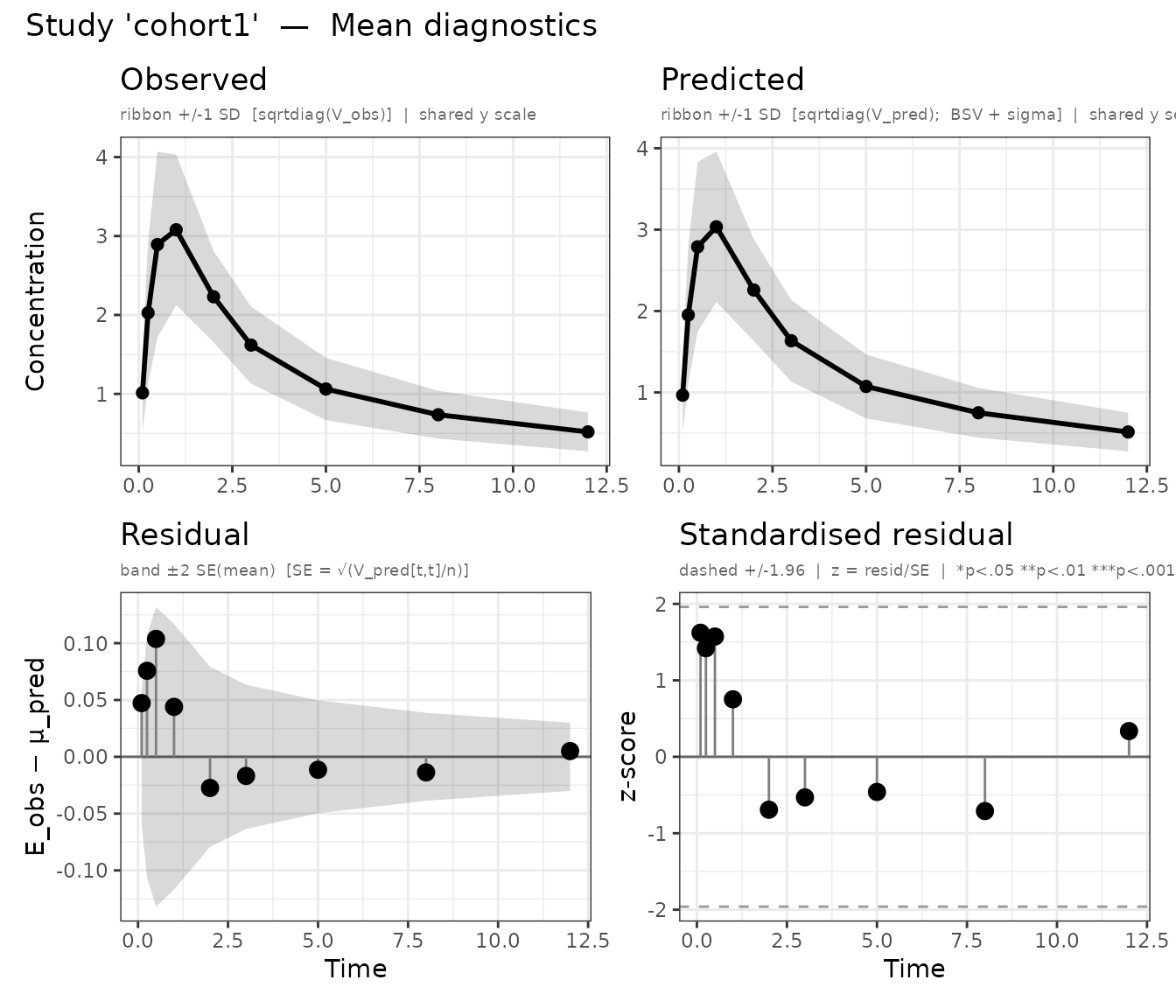
Mean diagnostics for both cohorts (one panel per study).
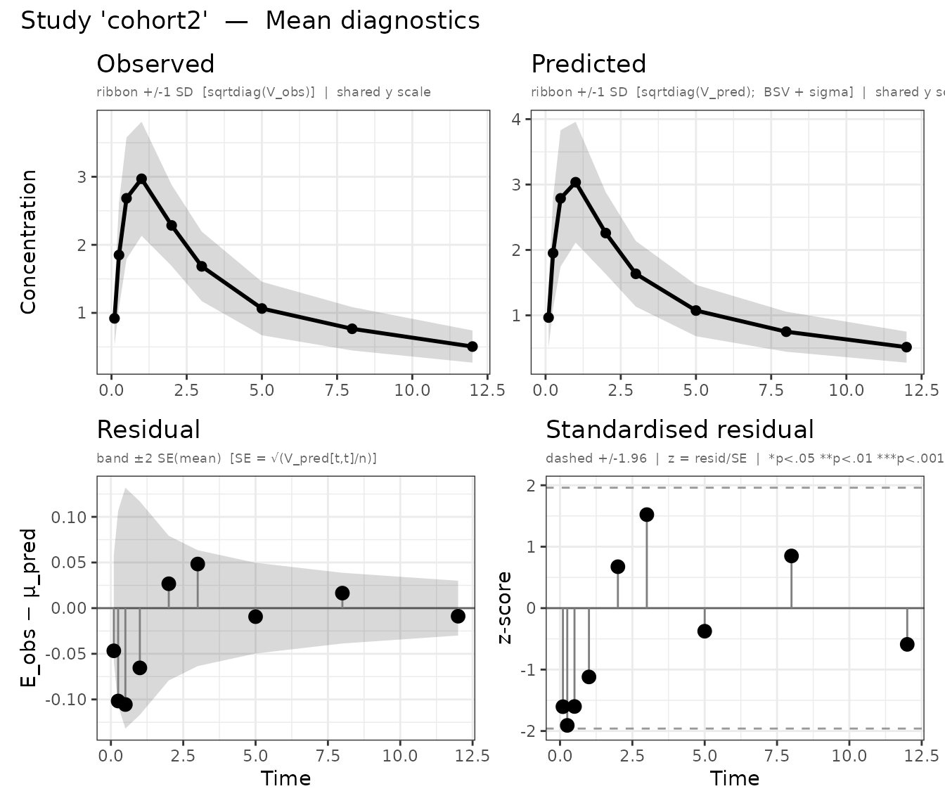
Mean diagnostics for both cohorts (one panel per study).
names(plots)
#> [1] "mean_cohort1" "mean_cohort2"
Access individual panels to compare studies side by side:
plots$mean_cohort1
plots$mean_cohort2

# Combine with patchwork if installed
if (requireNamespace("patchwork", quietly = TRUE)) {
  patchwork::wrap_plots(plots, ncol = 1)
}
Different doses and schedules
Studies may differ in any aspect. A typical multi-study setup from a drug development programme:
fit_program <- nlmixr2(
  pk_model, admData(), est = "admc",
  control = admControl(
    studies = list(
      phase1_50mg  = list(E = E_50,  V = V_50,  n = 30L,
                          times = c(1, 2, 4, 8),
                          ev    = rxode2::et(amt = 50)),
      phase2_100mg = list(E = E_100, V = V_100, n = 120L,
                          times = c(0.5, 1, 2, 4, 8, 12),
                          ev    = rxode2::et(amt = 100)),
      phase2_200mg = list(E = E_200, V = V_200, n = 115L,
                          times = c(0.5, 1, 2, 4, 8, 12),
                          ev    = rxode2::et(amt = 200))
    ),
    n_sim   = 5000L,
    maxeval = 1000L,
    seed    = 1L
  )
)
Studies with a diagonal V (or a plain vector of variances) are
automatically assigned method = "var", avoiding the O(n_t³)
Cholesky solve when the off-diagonal covariance structure is
unavailable.