Diagnostic plots for an admixr2 fit

Generates up to four diagnostic panels:

Usage

# S3 method for class 'admFit'
plot(x, which = c("mean", "cov", "nll", "par"), n_sim = NULL, seed = 1L, ...)

Arguments

x: An admFit object returned by nlmixr2() with est = "adfo", est = "admc", est = "adgh", or est = "adirmc".
which: Character vector selecting which panel types to produce. Any subset of c("mean", "cov", "nll", "par"). Defaults to all four.
n_sim: Number of MC samples for the final prediction. Defaults to the value used during fitting. Only used when "mean" or "cov" is in which.
seed: Random seed for reproducibility.
...: Unused.

Value

A named list of ggplot2 objects, invisibly. Prints each selected plot.

Details

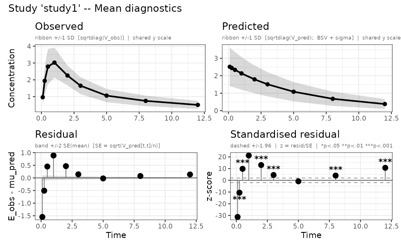
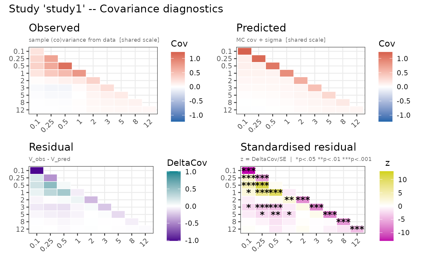
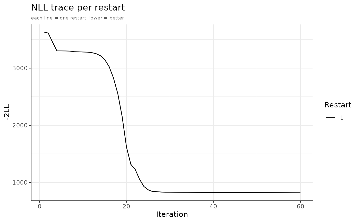
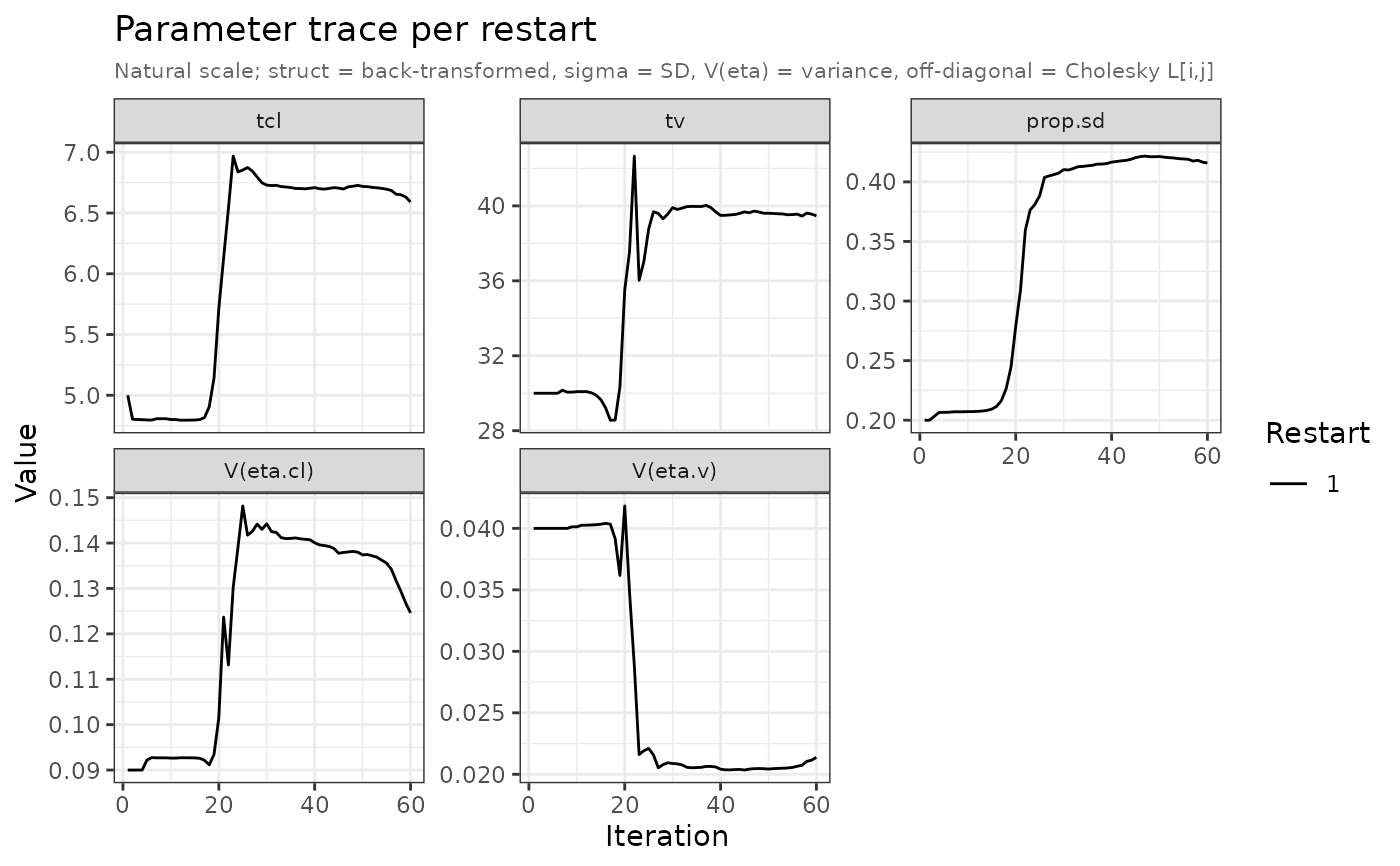
"mean" – Observed vs predicted mean per study (2x2 grid). Upper row: observed and predicted mean lines with +/-1 SD ribbon on a shared y scale (black throughout). Lower row: raw residual lollipop with +/-2 SE band and standardised residual z-scores with +/-1.96 reference lines.
"cov" – Observed vs predicted (co)variance heatmaps per study (2x2 grid). Upper row shares a common colour scale (blue-white-red). Lower row uses distinct diverging scales: residual (red-white-green) and standardised residual (gold-white-purple). Significance stars overlaid on the standardised residual panel.
"nll" – NLL trace per restart over optimizer evaluations. Restarts coloured with the Okabe-Ito palette.
"par" – Parameter trace per restart on the natural scale (struct thetas back-transformed, sigma as SD, omega diagonal as variance labelled V(eta.x)). Facets ordered as in the model ini() block. Restarts coloured with the Okabe-Ito palette.

nlmixr2 `traceplot()`

admixr2 fits also plug into the nlmixr2 traceplot() generic. During fitting the parameter iteration history of the best restart is stored on the fit in the standard parHistData slot (natural scale), so traceplot(fit) produces the familiar per-parameter, free-y facetted trace used elsewhere in the nlmixr2 ecosystem. There is no burn-in marker (admixr2 records optimizer evaluations, not SAEM iterations), and only the best restart is shown – the per-restart overlay and the NLL trace remain available via plot(fit, which = c("par", "nll")). The trace stores only improving evaluations (steps that lowered the best NLL), so the iter axis indexes those improvement steps rather than raw optimizer iterations.

Examples

# \donttest{
library(rxode2)
library(nlmixr2)

data("examplomycin")
obs    <- examplomycin[examplomycin$EVID == 0, ]
obs    <- obs[order(obs$ID, obs$TIME), ]
times  <- sort(unique(obs$TIME))
ids    <- unique(obs$ID)
dv_mat <- do.call(rbind, lapply(ids, function(i) {
  sub <- obs[obs$ID == i, ]; sub$DV[order(sub$TIME)]
}))
E <- colMeans(dv_mat)
V <- cov.wt(dv_mat, method = "ML")$cov

pk_model <- function() {
  ini({
    tcl <- log(5); tv <- log(30)
    prop.sd <- c(0, 0.2)
    eta.cl ~ 0.09; eta.v ~ 0.04
  })
  model({
    cl <- exp(tcl + eta.cl)
    v  <- exp(tv  + eta.v)
    d/dt(central) <- -(cl/v) * central
    cp <- central / v
    cp ~ prop(prop.sd)
  })
}

fit <- nlmixr2(
  pk_model, admData(), est = "adfo",
  control = adfoControl(
    studies = list(study1 = list(E = E, V = V, n = length(ids),
                                 times = times, ev = et(amt = 100))),
    maxeval = 100L
  )
)
#>  
#>  
#>  
#>  
#> ℹ parameter labels from comments are typically ignored in non-interactive mode
#> ℹ Need to run with the source intact to parse comments
#> === admixr2: Aggregate Data Modeling (FO) ===
#>   Studies: 1 | Params: 5 | Cores: 1 | Grad: none | Restarts: 1
#> +----------+----------+----------+----------+----------+----------+----------+
#> |          |     -2LL |      tcl |       tv |  prop.sd |   eta.cl |    eta.v |
#> +----------+----------+----------+----------+----------+----------+----------+
#> | 0010     |  1.5e+30 |        5 |        1 |      0.2 |     0.09 |     0.04 |
#> | 0020     |  3878.99 |    4.803 |    31.64 |      0.2 |     0.09 |     0.04 |
#> | 0030     |  3303.72 |    4.806 |     30.1 |   0.2068 |  0.09261 |     0.04 |
#> | 0040     |  2828.60 |    4.816 |    28.56 |   0.2164 |  0.09217 |  0.04034 |
#> | 0050     |   929.13 |    6.839 |    37.04 |   0.3811 |   0.1391 |  0.02192 |
#> | 0060     |   833.01 |    6.862 |    39.38 |   0.4076 |   0.1484 |  0.02135 |
#> | 0070     |   826.48 |    6.702 |    39.97 |   0.4139 |   0.1411 |  0.02057 |
#> | 0080     |   822.02 |    6.697 |    39.52 |   0.4177 |   0.1395 |  0.02036 |
#> | 0090     |   821.28 |    6.719 |    39.61 |   0.4213 |   0.1374 |  0.02043 |
#> | 0100     |   820.07 |     6.65 |    39.62 |   0.4181 |   0.1294 |  0.02105 |
#> | 0102 ✓   |   819.71 |    6.591 |    39.47 |   0.4158 |   0.1246 |  0.02138 |
#> | 3.8 sec  |          |          |          |          |          |          |
#>   Computing covariance (R method, 19 NLL evaluations)
#>   Note: covMethod='r' computes covariance for structural and sigma parameters only; omega (IIV) SEs are not computed (matching nlmixr2 FOCEI behavior).
#> → compress origData in nlmixr2 object, save 1160
plot(fit)
#>  
#>  




# }