From a published figure to E, V and n

The problem

Every study passed to admControl() needs a mean vector E, a covariance V, a sample size n, the observation times and a dosing event table ev. A published figure gives you a mean and an error bar.

Reading the mean off is easy. Getting the variance right is where aggregate analyses go wrong: a standard error used as a standard deviation is off by a factor of sqrt(n), and the fit does not tell you — the structural parameters come back correct and only the between-subject variability collapses. This vignette converts a published figure into E, V and n, and shows what that mistake costs.

library(admixr2)
library(rxode2)
library(nlmixr2)
library(ggplot2)

What V must be

V is the spread across subjects, not the precision of the mean. admixr2’s likelihood is

$-2LL = n \left( \log|V_{pred}| + \mathrm{tr}(V_{pred}^{-1} V_{obs}) + r^{\top} V_{pred}^{-1} r \right)$

where r is the mismatch between observed and predicted means, and V_pred = J Omega J' + Sigma — one subject’s covariance, built from the between-subject variability and the residual error. V_obs must be the same object, and the sample size n sits outside it. Hand the likelihood a standard error squared and you have told it about n twice.

So V = SD^2, never SEM^2.

What is the error bar?

Read the caption. If it does not say, treat the error bar as unknown rather than assuming:

Figure reports	Convert to SD	Note
Standard deviation (SD)	`SD`	Use directly
Standard error (SEM)	`SD = SEM * sqrt(n)`	Off by `sqrt(n)` if confused
95% CI of the mean	`SD = (upper - lower) * sqrt(n) / 3.92`	3.92 = 2 × 1.96; for small `n` use `2 * qt(0.975, n - 1)`
Interquartile range	`SD ~ IQR / 1.35`	Assumes normality
LS-mean SE (from an MMRM)	`SD ~ SE * sqrt(n)`	Biased small — see below

sd_from_sem <- function(sem, n)        sem * sqrt(n)
sd_from_ci  <- function(lower, upper, n) (upper - lower) * sqrt(n) / (2 * qt(0.975, n - 1))
sd_from_iqr <- function(q1, q3)        (q3 - q1) / 1.35

An LS-mean SE deserves care because it is the one row that can silently reproduce the error this vignette is about. It comes out of a model, usually an MMRM: baseline and covariate adjustment remove variance from the residual, and the covariance structure borrows across visits, so SE * sqrt(n) is usually smaller than the true between-subject SD — the same direction as mistaking a SEM for an SD. It also describes whatever the MMRM modelled, often a change from baseline rather than an absolute value. Prefer a descriptive SD from the paper’s own baseline table, or from a comparable study.

A figure reporting standard errors

A 50 mg arm, 60 subjects, digitised from a concentration–time figure whose caption reads “mean ± SEM” — the same arm used in PD and PK/PD data, before it was fitted:

times <- c(0.5, 1, 2, 4, 8, 12, 24)
E     <- c(0.969, 0.920, 0.831, 0.679, 0.460, 0.317, 0.111)     # mg/L
SEM   <- c(0.0267, 0.0243, 0.0205, 0.0161, 0.0137, 0.0125, 0.0080)
n     <- 60L

SD <- sd_from_sem(SEM, n)
round(SD, 3)
#> [1] 0.207 0.188 0.159 0.125 0.106 0.097 0.062

The bars the figure plots are sqrt(n) — nearly eight times — smaller than the standard deviations the fit needs. Plotting both makes it concrete: the SEM band is far too tight to be a between-subject spread.

band <- rbind(
  data.frame(t = times, m = E, lo = E - SD,  hi = E + SD,  what = "mean ± SD (what V needs)"),
  data.frame(t = times, m = E, lo = E - SEM, hi = E + SEM, what = "mean ± SEM (what the figure plots)"))

ggplot(band, aes(t, m)) +
  geom_ribbon(aes(ymin = lo, ymax = hi, fill = what), alpha = 0.25) +
  geom_line(linewidth = 0.9, colour = "grey20") +
  geom_point(size = 1.8, colour = "grey20") +
  facet_wrap(~ what) +
  scale_fill_manual(values = c("mean ± SD (what V needs)"          = "#0072B2",
                               "mean ± SEM (what the figure plots)" = "#D55E00"),
                    guide = "none") +
  labs(x = "Time (h)", y = "Concentration (mg/L)") +
  theme_minimal(base_size = 12) +
  theme(panel.grid.minor = element_blank(),
        strip.text = element_text(face = "bold", size = 10))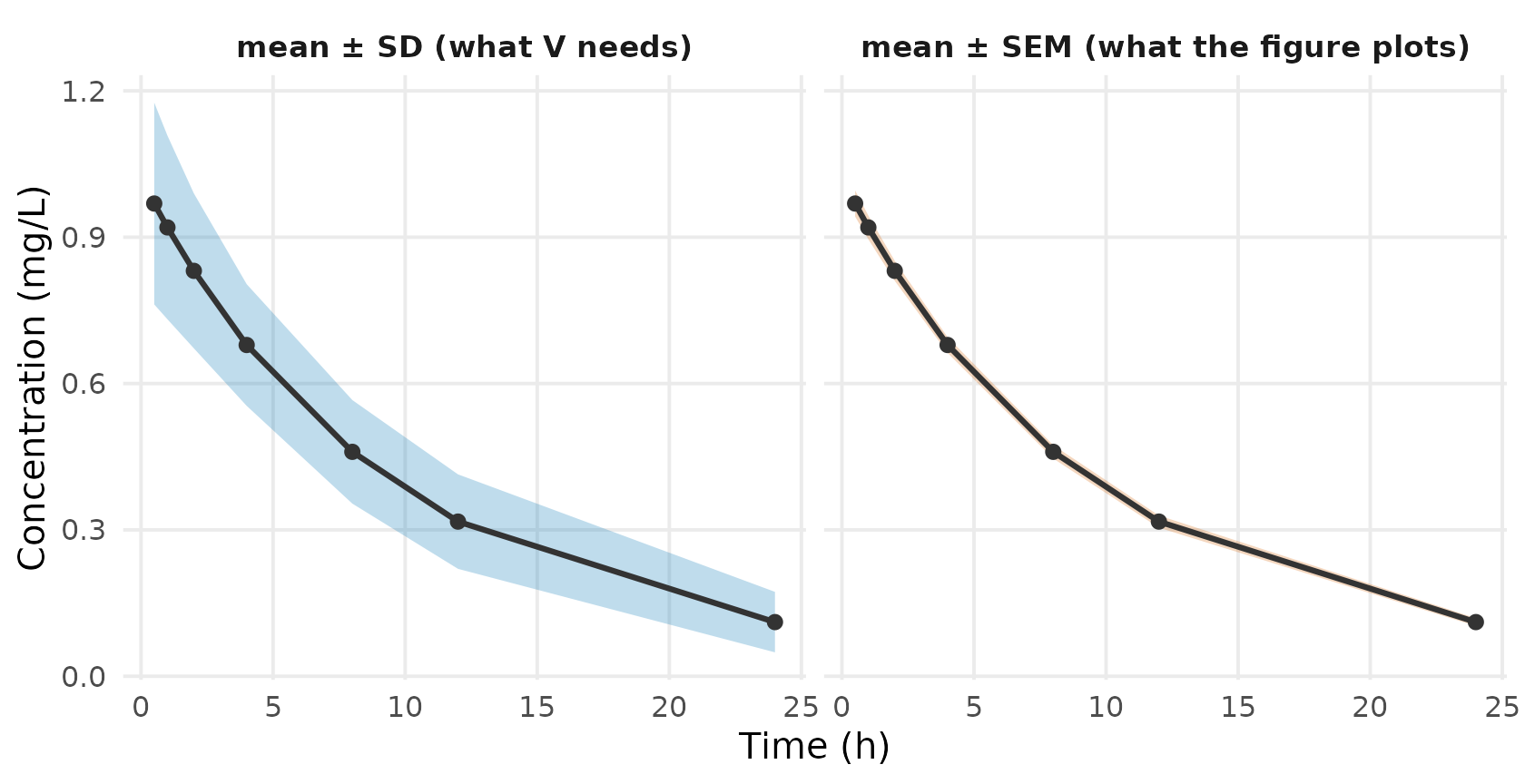

Passing V as a plain vector of variances is enough; admixr2 expands it to a diagonal matrix and sets method = "var":

study <- list(E = E, V = SD^2, n = n, times = times,
              ev = rxode2::et(amt = 50, cmt = "central"))

pk_model <- function() {
  ini({
    tcl <- log(4)  ; label("Log clearance (L/h)")
    tv  <- log(40) ; label("Log volume (L)")
    prop.cp <- 0.1 ; label("Proportional residual error")
    eta.cl ~ 0.09
    eta.v  ~ 0.04
  })
  model({
    cl <- exp(tcl + eta.cl)
    v  <- exp(tv  + eta.v)
    d/dt(central) <- -(cl/v) * central
    cp <- central / v
    cp ~ prop(prop.cp)
  })
}

fit <- nlmixr2(pk_model, admData(), est = "adgh",
               control = adghControl(studies = list(mg50 = study)))
fit
── nlmixr² adgh ──

          OBJF       AIC       BIC Log-likelihood
adgh -1323.146 -1313.146 -1292.945       661.5729

── Time (sec fit$time): ──

        optimize covariance elapsed other
elapsed    0.226      0.058   0.284  3.74

── Population Parameters (fit$parFixed or fit$parFixedDf): ──

                          Parameter    Est.      SE   %RSE
tcl             Log clearance (L/h)   1.556 0.01954  1.256
tv                   Log volume (L)   3.911 0.01546 0.3953
prop.cp Proportional residual error 0.09764               
        Back-transformed(95%CI) BSV(CV%) Shrink(SD)%
tcl         4.738 (4.56, 4.923)     25.9            
tv          49.96 (48.47, 51.5)     19.7            
prop.cp                 0.09764                     
 
  Covariance Type (fit$covMethod): r
  No correlations in between subject variability (BSV) matrix
  Full BSV covariance (fit$omega) or correlation (fit$omegaR; diagonals=SDs) 
  Distribution stats (mean/skewness/kurtosis/p-value) available in fit$shrink 
  Censoring (fit$censInformation): No censoring
  Minimization message (fit$message):  
    NLOPT_XTOL_REACHED: Optimization stopped because xtol_rel or xtol_abs (above) was reached.

What reading SEM as SD costs

Now make the mistake: use the plotted SEM as if it were an SD, so V is n-fold too small.

fit_wrong <- nlmixr2(
  pk_model, admData(), est = "adgh",
  control = adghControl(studies = list(
    mg50 = list(E = E, V = SEM^2, n = n, times = times,   # WRONG: SEM^2 as V
                ev = rxode2::et(amt = 50, cmt = "central")))))
fit_wrong
── nlmixr² adgh ──

          OBJF       AIC       BIC Log-likelihood
adgh -2942.661 -2932.661 -2912.459        1471.33

── Time (sec fit_wrong$time): ──

  optimize covariance elapsed
1    0.644       0.05   0.694

── Population Parameters (fit_wrong$parFixed or fit_wrong$parFixedDf): ──

                          Parameter     Est.       SE    %RSE
tcl             Log clearance (L/h)    1.558 0.003064  0.1967
tv                   Log volume (L)    3.908 0.002122 0.05431
prop.cp Proportional residual error 0.008208                 
        Back-transformed(95%CI) BSV(CV%) Shrink(SD)%
tcl         4.749 (4.72, 4.777)     4.19            
tv         49.78 (49.57, 49.99)     2.91            
prop.cp                0.008208                     
 
  Covariance Type (fit_wrong$covMethod): r
  No correlations in between subject variability (BSV) matrix
  Full BSV covariance (fit_wrong$omega) 
    or correlation (fit_wrong$omegaR; diagonals=SDs)
  Distribution stats (mean/skewness/kurtosis/p-value) available in $shrink 
  Censoring (fit_wrong$censInformation): No censoring
  Minimization message (fit_wrong$message):  
    NLOPT_XTOL_REACHED: Optimization stopped because xtol_rel or xtol_abs (above) was reached.

Clearance and volume are unchanged to three figures. The between-subject variability is not:

round(diag(fit$omega) / diag(fit_wrong$omega), 1)
#> eta.cl  eta.v 
#>   36.9   45.3

Omega shrinks by more than an order of magnitude on both random effects, because the model is asked to reproduce a between-subject spread n times tighter than the real one. V_pred = J Omega J' + Sigma is linear in Omega and in the residual variance, so both shrink together and the structural parameters are free to stay where they were. The shrinkage stops short of the full factor of n only because the mean-mismatch term r' V_pred^-1 r does not rescale.

Nothing in the point estimates warns you. The precision does:

round(c(RSE_CL_correct = fit$parFixedDf["tcl", "%RSE"],
        RSE_CL_wrong   = fit_wrong$parFixedDf["tcl", "%RSE"]), 3)
#> RSE_CL_correct   RSE_CL_wrong 
#>          1.256          0.197

Clearance comes back not just right but implausibly certain — its standard error tightens about 6.4-fold, of order sqrt(n). An RSE that looks too good for digitised literature data, or an IIV that comes back near zero, is the tell.

Two things make this worse than the demo suggests:

The structural parameters only survive because this model fits. With a misspecified model, r is not zero, and a V_pred that is n times too small weights that mismatch n times too heavily — dragging the structural estimates to close a gap they cannot close.
In a multi-study fit, one bad V captures the whole fit. Getting V wrong in a single study inflates that study’s weight in the joint likelihood roughly n-fold. It then dominates every other arm and biases the shared parameters. This is the usual way admixr2 is used, and it is where the mistake is most expensive.

Why V is usually diagonal

A figure gives one error bar per time point and nothing about how the times covary, so the off-diagonal entries of V are not available from published summaries. A diagonal V selects method = "var", which skips the Cholesky solve the full-covariance path needs. This is the honest default for literature data. The full-covariance path is available when you have the subject-level matrix and can compute cov.wt(dv_mat, method = "ML")$cov — see Getting started.

Note the denominator. admixr2’s likelihood wants the ML (n) variance, while a published SD is the unbiased (n - 1) sample SD, so strictly V = SD^2 * (n - 1) / n. At n = 60 that is a 1.7% change and is usually ignored; below n of about 15 it is worth applying. The method = "ML" rule matters most when you compute V yourself from subject-level data.

Sample size

n is the number of subjects contributing to the summary, per arm — not the total across arms, and not the number of observations.

Dropout. n often falls over time, so a figure’s late points may rest on fewer subjects than its early ones. Convert each point’s error bar with the n that applies to it, and pass the number contributing to the observations you are fitting — the number at risk, not the number randomised.
Per-endpoint n. PK and PD are not always measured in the same people. A study’s observations entries may each carry their own n.

Absolute values or change from baseline?

Many PD papers report a least-squares-mean change from baseline rather than an absolute value. Either can be fitted, but the model must predict the same quantity as the data:

Fitting absolute values needs a baseline parameter in the model; see PD and PK/PD data.
Fitting a change means the model output must itself be a change, and the SD of the change — not of the absolute value — is the one V needs.

Studies that report different quantities must be converted to a common one before fitting, not after.

When there is no variability at all

A paper often gives a mean with no SD, SEM or CI — a placebo arm reported only in a footnote, for example.

You then have to assume a V, and it is worth knowing what that assumption does. Refit the arm above with the SD deliberately wrong in each direction:

assume <- function(mult) {
  f <- nlmixr2(pk_model, admData(), est = "adgh",
               control = adghControl(studies = list(
                 mg50 = list(E = E, V = (SD * mult)^2, n = n, times = times,
                             ev = rxode2::et(amt = 50, cmt = "central")))))
  c(exp(f$theta[["tcl"]]), exp(f$theta[["tv"]]),
    diag(f$omega)[["eta.cl"]], diag(f$omega)[["eta.v"]])
}

mults <- c(0.5, 1, 2, 4)
res   <- t(vapply(mults, assume, numeric(4)))

tbl <- data.frame(
  `Assumed SD` = c("0.5x  (too small)", "1x  (correct)",
                   "2x  (too large)",   "4x  (too large)"),
  CL           = round(res[, 1], 2),
  V            = round(res[, 2], 2),
  `var(eta.cl)` = round(res[, 3], 3),
  `var(eta.v)`  = round(res[, 4], 3),
  check.names  = FALSE
)

knitr::kable(tbl, row.names = FALSE,
             caption = "Fit against a deliberately wrong V. Truth: CL = 5, V = 50, var(eta.cl) = 0.09, var(eta.v) = 0.04.")

Fit against a deliberately wrong V. Truth: CL = 5, V = 50, var(eta.cl) = 0.09, var(eta.v) = 0.04.
Assumed SD	CL	V	var(eta.cl)	var(eta.v)
0.5x (too small)	4.74	49.89	0.017	0.010
1x (correct)	4.74	49.96	0.065	0.038
2x (too large)	4.78	49.85	0.264	0.111
4x (too large)	1.82	0.85	0.029	5.937

Omega follows the assumption in whichever direction it is wrong: too small and the between-subject variability collapses, too large and it inflates several-fold. V is data the model must reproduce, not a weight — so an assumed V is an assumption about the IIV you are trying to estimate, and it propagates to every study through the shared Omega. Push it far enough and the fit stops being sensible at all: at 4x the structural parameters leave the building.

There is no safe direction to err in. In rough order of preference:

Take the variability from a comparable arm, or a comparable study of the same endpoint.
Use a published typical SD for that endpoint and population.
Exclude the study.

Whichever you choose, record it, and refit across the range you consider plausible. If the estimates move, the assumption is doing the work and the result belongs in a sensitivity table rather than a headline.

Notes

The error bar is the dominant error source. Digitisation software is accurate to a few percent; mistaking a SEM for an SD is an error of sqrt(n). Reading the caption matters more than the pixels.
Geometric means. A paper reporting a geometric mean and CV% is describing a log-normal distribution, while E and V are arithmetic moments. Convert before fitting.
Digitising. WebPlotDigitizer is the usual tool. Extracting a figure twice and comparing is a cheap check.
%RSE is on the estimation scale. These parameters are log-scale, so an RSE on tcl is not an RSE on clearance.
PD specifics — baselines, placebo arms, two endpoints — are covered in PD and PK/PD data.