When would you use datagen?
Two common situations call for generating aggregate data programmatically:
Simulation studies. You want to check that an
estimator recovers the true parameters. Define a data-generating model
with known parameters, call datagen() to obtain E and V,
fit your analysis model, and compare the estimates to the truth.
Literature-based modelling. Each published study was
analysed with its own structural PK model (possibly a different number
of compartments, a different parameterisation, or only a subset of the
IIV terms). datagen() lets each study carry its own model
so that the simulated aggregate data reflects the original authors’
model, not a single shared structure.
In both cases the output is a named list of
(E, V, n, times, ev) objects that plug directly into
admControl(studies = ...).
Simulation study: same model across studies
Here we use a one-compartment oral model to generate two synthetic
study datasets — a low-dose and a high-dose arm — then verify that
adfo recovers the true structural parameters.
Data-generating model
library(admixr2)
library(rxode2)
library(nlmixr2)
library(ggplot2)

true_model <- function() {
  ini({
    tcl     <- log(5)  ; label("Log clearance (L/h)")
    tv      <- log(10) ; label("Log volume (L)")
    tka     <- log(1)  ; label("Log absorption rate (1/h)")
    prop.sd <- c(0, 0.2) ; label("Proportional error SD")
    eta.cl  ~ 0.09
    eta.v   ~ 0.04
    eta.ka  ~ 0.04
  })
  model({
    cl <- exp(tcl + eta.cl)
    v  <- exp(tv  + eta.v)
    ka <- exp(tka + eta.ka)
    d/dt(depot)   <- -ka * depot
    d/dt(central) <- ka * depot - (cl/v) * central
    cp <- central / v
    cp ~ prop(prop.sd)
  })
}
True parameter values: CL = 5 L/h, V = 10 L, ka = 1 h⁻¹; IIV of 0.3 (SD on log scale) for CL and 0.2 for V and ka; proportional residual error SD = 0.2.
Generating the data
Pass the model as the top-level default so all studies inherit it.
Each study spec needs only times, ev, and
n:
times <- c(0.5, 1, 2, 4, 8, 12, 24)

study_data <- datagen(
  studies = list(
    low_dose  = list(times = times, ev = rxode2::et(amt =  50), n = 250L),
    high_dose = list(times = times, ev = rxode2::et(amt = 100), n = 250L)
  ),
  model   = true_model,
  control = datagenControl(n_sim = 10000L, seed = 1L)
)

# Each study returns E, V, n, times, ev
names(study_data$low_dose)
#> [1] "E"     "V"     "n"     "times" "ev"
round(study_data$low_dose$E, 2)   # population mean at each time
#>  0.5    1    2    4    8   12   24
#> 1.75 2.38 2.27 1.18 0.24 0.06 0.00
The covariance matrix V captures both IIV-driven
between-time correlation and the residual error contribution on the
diagonal:
round(study_data$low_dose$V, 3)
#>        0.5      1     2      4      8     12    24
#> 0.5  0.291  0.187 0.106 -0.005 -0.018 -0.007 0.000
#> 1    0.187  0.452 0.171  0.051  0.001 -0.001 0.000
#> 2    0.106  0.171 0.420  0.161  0.051  0.015 0.001
#> 4   -0.005  0.051 0.161  0.255  0.084  0.028 0.001
#> 8   -0.018  0.001 0.051  0.084  0.046  0.016 0.001
#> 12  -0.007 -0.001 0.015  0.028  0.016  0.007 0.000
#> 24   0.000  0.000 0.001  0.001  0.001  0.000 0.000
Inspecting the generated profiles
df_gen <- do.call(rbind, lapply(names(study_data), function(nm) {
  s  <- study_data[[nm]]
  sd <- sqrt(diag(s$V))
  data.frame(study = nm, time = s$times,
             mean = s$E, lo = s$E - sd, hi = s$E + sd)
}))

ggplot(df_gen, aes(x = time, y = mean, colour = study, fill = study)) +
  geom_ribbon(aes(ymin = lo, ymax = hi), alpha = 0.15, colour = NA) +
  geom_line(linewidth = 1) +
  geom_point(size = 2.5) +
  scale_x_log10(breaks = times, labels = times) +
  scale_colour_manual(values = c(low_dose = "#0072B2", high_dose = "#D55E00")) +
  scale_fill_manual(  values = c(low_dose = "#0072B2", high_dose = "#D55E00")) +
  labs(title  = "Generated aggregate data — mean ± 1 SD",
       x = "Time (h, log scale)", y = "Concentration (mg/L)",
       colour = NULL, fill = NULL) +
  theme_bw()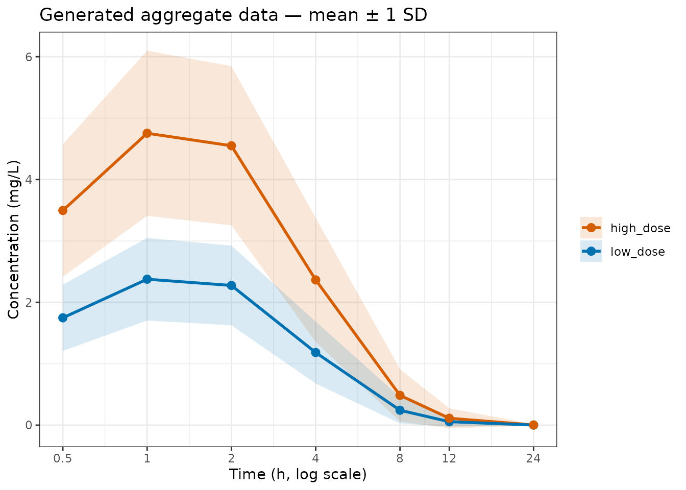
Generated population mean ± 1 SD for both dose levels.
The ribbon reflects the square root of the diagonal of V: IIV spread plus residual error. Off-diagonal entries (the within-subject correlation structure) are not shown but are passed to the estimator and used in the likelihood.
Parameter recovery
The generated data plug directly into
admControl(studies = ...). The analysis model is the same
structural model — this lets us verify estimator consistency:
analysis_model <- function() {
  ini({
    tcl     <- log(4)  ; label("Log clearance (L/h)")
    tv      <- log(12) ; label("Log volume (L)")
    tka     <- log(1.5); label("Log absorption rate (1/h)")
    prop.sd <- c(0, 0.3); label("Proportional error SD")
    eta.cl  ~ 0.12
    eta.v   ~ 0.05
    eta.ka  ~ 0.05
  })
  model({
    cl <- exp(tcl + eta.cl)
    v  <- exp(tv  + eta.v)
    ka <- exp(tka + eta.ka)
    d/dt(depot)   <- -ka * depot
    d/dt(central) <- ka * depot - (cl/v) * central
    cp <- central / v
    cp ~ prop(prop.sd)
  })
}
Starting values are deliberately offset from the truth (CL start = 4 vs true 5, V start = 12 vs true 10) to demonstrate that the estimator finds them regardless.
fit_sim <- nlmixr2(
  analysis_model, admData(), est = "admc",
  control = admControl(
    studies   = study_data,
    maxeval   = 300L,
    covMethod = "r"
  )
)
#> [====|====|====|====|====|====|====|====|====|====] 0:00:00
#> [====|====|====|====|====|====|====|====|====|====] 0:00:00
#> [====|====|====|====|====|====|====|====|====|====] 0:00:00
#> [====|====|====|====|====|====|====|====|====|====] 0:00:00
#> [====|====|====|====|====|====|====|====|====|====] 0:00:00
#> [====|====|====|====|====|====|====|====|====|====] 0:00:00
#>
#> [====|====|====|====|====|====|====|====|====|====] 0:00:00
#>
#> [====|====|====|====|====|====|====|====|====|====] 0:00:00
#> [====|====|====|====|====|====|====|====|====|====] 0:00:00
#> [====|====|====|====|====|====|====|====|====|====] 0:00:00
#> [====|====|====|====|====|====|====|====|====|====] 0:00:00
#> [====|====|====|====|====|====|====|====|====|====] 0:00:00
#> [====|====|====|====|====|====|====|====|====|====] 0:00:03
#>
#> [====|====|====|====|====|====|====|====|====|====] 0:00:03

print(fit_sim)
#> ── nlmixr² admc ──
#>
#>           OBJF       AIC       BIC Log-likelihood
#> admc -7889.378 -7875.378 -7832.254       3944.689
#>
#> ── Time (sec fit_sim$time): ──
#>
#>   optimize covariance elapsed
#> 1   65.256      7.761  73.017
#>
#> ── Population Parameters (fit_sim$parFixed or fit_sim$parFixedDf): ──
#>
#>                         Parameter     Est.       SE   %RSE
#> tcl           Log clearance (L/h)    1.608 0.009336 0.5806
#> tv                 Log volume (L)    2.303  0.01276 0.5543
#> tka     Log absorption rate (1/h) 0.001747  0.01798   1029
#> prop.sd     Proportional error SD   0.1999
#>         Back-transformed(95%CI) BSV(CV%) Shrink(SD)%
#> tcl        4.994 (4.903, 5.086)     30.4
#> tv            10 (9.754, 10.25)     19.6
#> tka       1.002 (0.9671, 1.038)     20.9
#> prop.sd                  0.1999
#>
#>   Covariance Type (fit_sim$covMethod): r
#>   No correlations in between subject variability (BSV) matrix
#>   Full BSV covariance (fit_sim$omega)
#>     or correlation (fit_sim$omegaR; diagonals=SDs)
#>   Distribution stats (mean/skewness/kurtosis/p-value) available in $shrink
#>   Censoring (fit_sim$censInformation): No censoring
#>   Minimization message (fit_sim$message):
#>     NLOPT_XTOL_REACHED: Optimization stopped because xtol_rel or xtol_abs (above) was reached.
Structural parameter estimates and the truth:
Literature workflow: per-study models
When digitising data from publications, each study comes with its own
model. A 2016 paper may have used a one-compartment model; a 2022
follow-up may have used two compartments. datagen() accepts
a model element inside each study spec that overrides the
top-level default:
# One-compartment oral model (as published in a simpler earlier study)
model_1cmt <- function() {
  ini({
    tcl     <- log(5)
    tv      <- log(40)    # apparent volume, peripheral compartment lumped in
    tka     <- log(1)
    prop.sd <- c(0, 0.25)
    eta.cl  ~ 0.04
    eta.v   ~ 0.01
    eta.ka  ~ 0.01
  })
  model({
    cl <- exp(tcl + eta.cl)
    v  <- exp(tv  + eta.v)
    ka <- exp(tka + eta.ka)
    d/dt(depot)   <- -ka * depot
    d/dt(central) <- ka * depot - (cl/v) * central
    cp <- central / v
    cp ~ prop(prop.sd)
  })
}

# Two-compartment oral model (as published in a more detailed later study)
model_2cmt <- function() {
  ini({
    tcl     <- log(5)
    tv1     <- log(10)
    tv2     <- log(30)
    tq      <- log(10)
    tka     <- log(1)
    prop.sd <- c(0, 0.2)
    eta.cl  ~ 0.09
    eta.v1  ~ 0.04
  })
  model({
    cl <- exp(tcl + eta.cl)
    v1 <- exp(tv1 + eta.v1)
    v2 <- exp(tv2)
    q  <- exp(tq)
    ka <- exp(tka)
    d/dt(depot)      <- -ka * depot
    d/dt(central)    <- ka * depot - (cl/v1 + q/v1) * central + (q/v2) * peripheral
    d/dt(peripheral) <- (q/v1) * central - (q/v2) * peripheral
    cp <- central / v1
    cp ~ prop(prop.sd)
  })
}
Both studies share the same CL (5 L/h) but differ in how they describe distribution: the earlier study lumped peripheral distribution into a single larger apparent volume (V = 15 L), while the later study resolved the two compartments (V₁ = 10 L, V₂ = 30 L, Q = 10 L/h).
lit_data <- datagen(
  studies = list(
    early_study = list(
      model = model_1cmt,
      times = c(0.5, 1, 2, 4, 8, 12),
      ev    = rxode2::et(amt = 100),
      n     = 120L
    ),
    later_study = list(
      model = model_2cmt,
      times = c(2, 4, 8, 12, 24),
      ev    = rxode2::et(amt = 200),
      n     = 180L
    )
  ),
  control = datagenControl(n_sim = 10000L, seed = 2L)
)
The two studies share the same drug (same CL) but have different E profiles because of the different dosing and distributional assumptions:
df_lit <- do.call(rbind, lapply(names(lit_data), function(nm) {
  s  <- lit_data[[nm]]
  sd <- sqrt(diag(s$V))
  data.frame(study = nm, time = s$times,
             mean = s$E, lo = s$E - sd, hi = s$E + sd)
}))

ggplot(df_lit, aes(x = time, y = mean, colour = study, fill = study)) +
  geom_ribbon(aes(ymin = lo, ymax = hi), alpha = 0.15, colour = NA) +
  geom_line(linewidth = 1) +
  geom_point(size = 2.5) +
  scale_colour_manual(values = c(early_study = "#009E73", later_study = "#CC79A7")) +
  scale_fill_manual(  values = c(early_study = "#009E73", later_study = "#CC79A7")) +
  labs(title  = "Literature-derived aggregate profiles",
       x = "Time (h)", y = "Concentration (mg/L)",
       colour = NULL, fill = NULL) +
  theme_bw()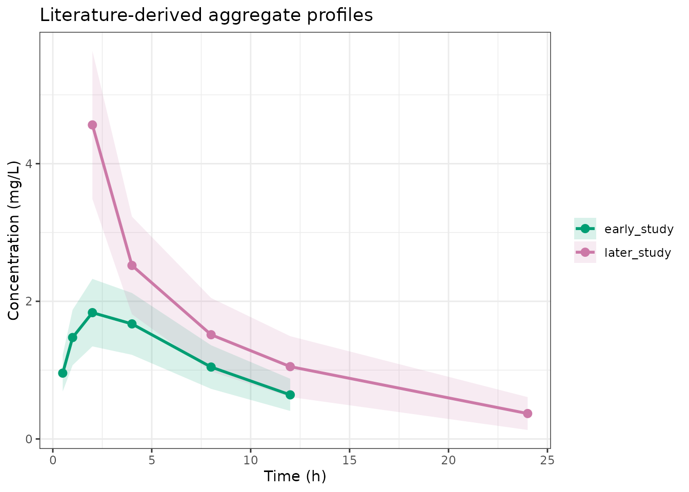
Simulated aggregate profiles from two publications with different structural models.
Fitting an analysis model to literature data
The data-generating models encode each publication’s assumptions; the analysis model represents your unified structural hypothesis. Here we fit the two-compartment oral model to both studies jointly:
lit_analysis <- function() {
  ini({
    tcl     <- log(5)
    tv1     <- log(10)
    tv2     <- log(30)
    tq      <- log(10)
    tka     <- log(1)
    prop.sd <- c(0, 0.25)
    eta.cl  ~ 0.09
    eta.v1  ~ 0.04
  })
  model({
    cl <- exp(tcl + eta.cl)
    v1 <- exp(tv1 + eta.v1)
    v2 <- exp(tv2)
    q  <- exp(tq)
    ka <- exp(tka)
    d/dt(depot)      <- -ka * depot
    d/dt(central)    <- ka * depot - (cl/v1 + q/v1) * central + (q/v2) * peripheral
    d/dt(peripheral) <- (q/v1) * central - (q/v2) * peripheral
    cp <- central / v1
    cp ~ prop(prop.sd)
  })
}

fit_lit <- nlmixr2(
  lit_analysis, admData(), est = "admc",
  control = admControl(
    studies   = lit_data,
    n_sim     = 5000L,
    cov_n_sim = 10000L,
    seed      = 3L
  )
)
Because the two studies used genuinely different structural models, the analysis model will find parameter values that minimise the joint discrepancy between its predictions and both studies’ aggregate data — a weighted compromise across the two parameterisations. This is expected behaviour: aggregate-data modelling accepts that each study was published under a different structural assumption and seeks a unified set of parameters that is consistent with all of them.
Examining individual simulated samples
Set return_samples = TRUE in
datagenControl() to include the raw
n_sim × n_times prediction matrix in each study’s output.
This is useful for inspecting the shape of the simulated distribution or
for constructing custom summaries:
study_with_samples <- datagen(
  studies = list(
    single_study = list(times = times, ev = rxode2::et(amt = 100), n = 250L)
  ),
  model   = true_model,
  control = datagenControl(n_sim = 2000L, seed = 4L, return_samples = TRUE)
)

cp_mat <- study_with_samples$single_study$samples   # 2000 x 7
mu     <- study_with_samples$single_study$E

df_samp <- data.frame(
  time  = rep(times, each = 200),
  conc  = as.vector(cp_mat[1:200, ]),
  id    = rep(seq_len(200), times = length(times))
)

ggplot(df_samp, aes(x = time, y = conc, group = id)) +
  geom_line(alpha = 0.06, colour = "grey30") +
  geom_line(data = data.frame(time = times, conc = mu),
            aes(group = NULL), colour = "#0072B2", linewidth = 1.5) +
  labs(title = "Simulated individual trajectories (n = 200 shown)",
       x = "Time (h)", y = "Concentration (mg/L)") +
  theme_bw()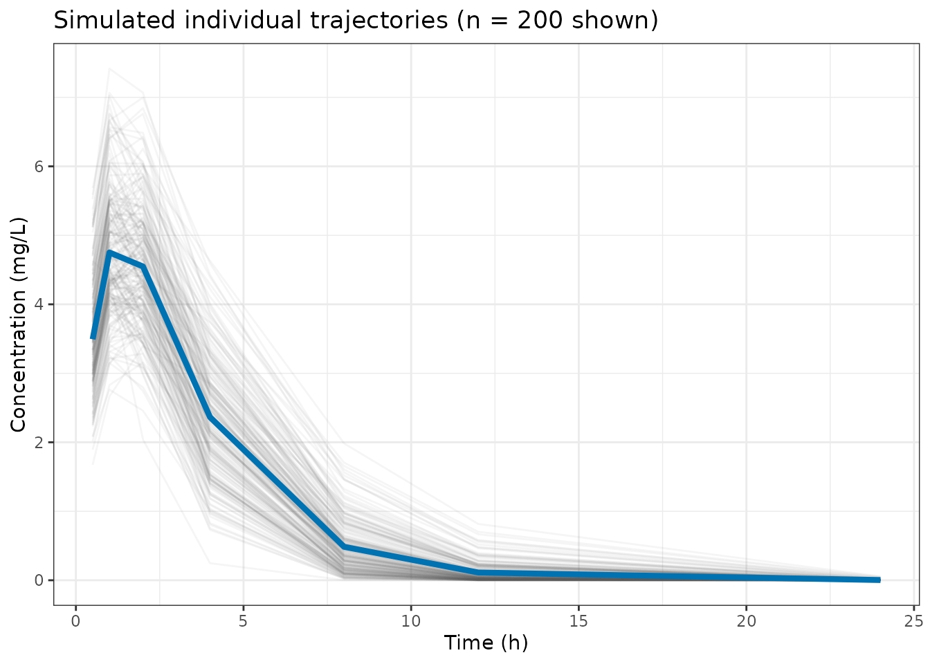
First 200 individual simulated trajectories (grey) with the population mean (blue).
The blue line is the population mean E; the grey spaghetti shows the
IIV spread. Note that samples contains concentrations
before residual error is added; the diagonal of V
additionally carries the residual error variance.
First-Order moments for design evaluation
By default datagen() integrates over the IIV
distribution by Monte Carlo, the same engine as
est = "admc". For design evaluation and optimal-design work
it is often preferable to generate E and V
from the deterministic First-Order expansion instead, which is what
est = "adfo" uses:
Switch with method = "fo" in
datagenControl():
fo_data <- datagen(
  studies = list(
    single_study = list(times = times, ev = rxode2::et(amt = 100), n = 250L)
  ),
  model   = true_model,
  control = datagenControl(method = "fo")
)

round(fo_data$single_study$E, 3)
#>   0.5     1     2     4     8    12    24
#> 3.445 4.773 4.651 2.340 0.360 0.049 0.000
There are two reasons to prefer FO here. First, the moments are
deterministic and fast — no n_sim, sampling or
seed (those arguments are ignored), so the result is
exactly reproducible. Second, and more importantly, it keeps the
data-generating and data-analytic models identical: when you
subsequently take the Hessian of the FO log-likelihood at the generating
parameters (the expected information matrix), it is evaluated at a
genuine maximum. If you generate with Monte Carlo and then analyse under
FO, the generating parameters are not in general an FO maximum
likelihood estimate of those data, and the resulting FIM is biased. So
for FIM / optimal-design calculations, generate and analyse with the
same FO approximation.
Gauss-Hermite moments for design evaluation with adgh
method = "fo" matches est = "adfo" but
inherits FO’s bias for nonlinear models or large IIV. The GH method
provides a deterministic, noise-free alternative that is
unbiased at any IIV magnitude and matches the moments
computed by est = "adgh":
where
are the
tensor-product Gauss-Hermite nodes and weights (Cholesky-scaled to the
current
).
Like method = "fo" the result is exact and reproducible —
no stochastic sampling. Use method = "gh" together with
est = "adgh" for design evaluation and optimal-design work
when FO bias would be non-negligible:
gh_data <- datagen(
  studies = list(
    single_study = list(times = times, ev = rxode2::et(amt = 100), n = 250L)
  ),
  model   = true_model,
  control = datagenControl(method = "gh", n_nodes = 5L)
)

round(gh_data$single_study$E, 3)
#>   0.5     1     2     4     8    12    24
#> 3.495 4.753 4.549 2.365 0.485 0.113 0.003
The MC, FO and GH means should agree closely when IIV is moderate and
the model is nearly linear in
.
GH and FO diverge from MC as IIV grows — GH tracks MC more accurately
because it does not linearise
.
The number of nodes n_nodes (per eta dimension) trades
accuracy against computational cost: n_nodes = 3 is fast;
n_nodes = 5 (default) achieves near-exact moments for IIV
SD up to ~0.5; n_nodes = 7 extends coverage to SD ~0.7.