Choosing a residual error model

The question

Your model ends with cp ~ prop(res.sd), as in an individual-level fit. The input is not individual data, though. It is a mean and an error bar per time point, digitised from a published figure or implied by a published model you supplied through datagen() — and usually several studies of them at once.

Each error bar holds two things the fit has to tell apart: subjects genuinely differ from one another, and each reported value carries variability the structural model does not explain. Your residual model is the claim about how to split them, and that split decides what goes to omega and what to the residual.

library(admixr2)
library(rxode2)
library(nlmixr2)
library(ggplot2)

How residual error lives in aggregate data

An error bar in a published figure is one number covering two sources of spread: subjects differ from one another, and each reported value carries variability the structural model does not explain. Only the second is your residual model’s job.

Everything below uses one model and one study. datagen() stands in for a digitised summary here so that the true values are known; a real analysis would read E, V and n off the paper — see From a published figure to E, V and n.

times <- c(0.5, 1, 2, 4, 8, 12, 24)

mod_prop <- function() {
  ini({
    tcl     <- log(5)   ; label("Log clearance (L/h)")
    tv      <- log(20)  ; label("Log volume (L)")
    res.sd  <- c(0, 0.2); label("Residual error SD")
    eta.cl  ~ 0.09
    eta.v   ~ 0.04
  })
  model({
    cl <- exp(tcl + eta.cl)
    v  <- exp(tv  + eta.v)
    d/dt(central) <- -(cl / v) * central
    cp <- central / v
    cp ~ prop(res.sd)
  })
}

gen <- datagen(
  studies = list(s1 = list(times = times, ev = rxode2::et(amt = 100), n = 200L)),
  model = mod_prop, control = datagenControl(n_sim = 20000L, seed = 1L))

Simulating the individual data behind such a summary — 20 000 subjects, each observed 25 times so that the two sources can be separated — shows how the two parts sit inside the error bar:

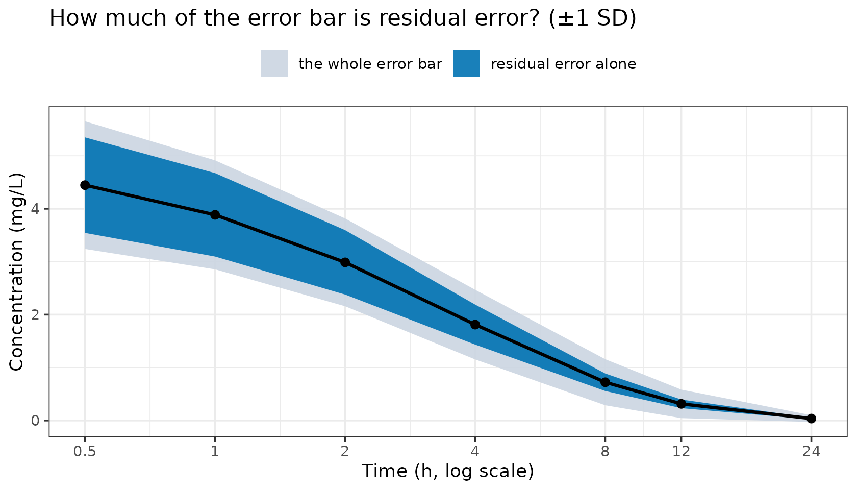
The light band is the whole error bar; the dark band is how much of it residual error alone would produce. The dark band is drawn inside the light one, not stacked on it: the total SD is sqrt(var_between + var_resid), not the sum of the two SDs.

The residual’s share of the error bar is not constant: it dominates early and is almost invisible by 24 h. That changing share is the shape information a fit uses to tell the two apart, which is why the residual model you name matters and why a wrong one has somewhere to hide.

What a wrong residual model does to a fit

Fit the same study twice, changing only the error line:

mod_add <- mod_prop |> model(cp ~ add(res.sd)) |> ini(res.sd = 0.5)

fit_prop <- nlmixr2(mod_prop, admData(), est = "adgh",
                    control = adghControl(studies = gen, print = 0L))
fit_add  <- nlmixr2(mod_add,  admData(), est = "adgh",
                    control = adghControl(studies = gen, print = 0L))

pull <- function(fit, nm) unname(fit$parFixedDf[nm, "Estimate"])

knitr::kable(
  data.frame(
    parameter = c("CL (L/h)", "V (L)", "IIV on CL", "IIV on V",
                  "residual SD", "-2LL"),
    truth     = c(5, 20, 0.09, 0.04, 0.2, NA),
    prop      = c(exp(pull(fit_prop, "tcl")), exp(pull(fit_prop, "tv")),
                  fit_prop$omega[1, 1], fit_prop$omega[2, 2],
                  pull(fit_prop, "res.sd"), fit_prop$objective),
    add       = c(exp(pull(fit_add, "tcl")),  exp(pull(fit_add, "tv")),
                  fit_add$omega[1, 1],  fit_add$omega[2, 2],
                  pull(fit_add, "res.sd"),  fit_add$objective)),
  digits = 3,
  caption = paste("Same data, same structural model, two residual models.",
                  "The additive residual SD is in mg/L and is not comparable to",
                  "the proportional one."))

Same data, same structural model, two residual models. The additive residual SD is in mg/L and is not comparable to the proportional one.
parameter	truth	prop	add
CL (L/h)	5.00	5.002	5.213
V (L)	20.00	19.996	19.597
IIV on CL	0.09	0.090	0.084
IIV on V	0.04	0.040	0.065
residual SD	0.20	0.200	0.467
-2LL	NA	-1542.269	-4.118

The proportional fit recovers all five generating values. The additive fit leaves clearance and volume within a few percent, which is the dangerous part, since CL and V are usually the first numbers anyone checks. Meanwhile the IIV on volume comes back 63% too large: the variance the residual failed to account for has to go somewhere, and a trial sized from that fit would simulate the wrong spread.

The objective moves 1538 points, so comparing the two fits catches it. The covariance panel shows the same thing without needing a second fit to compare against:

plot(fit_add, which = "cov")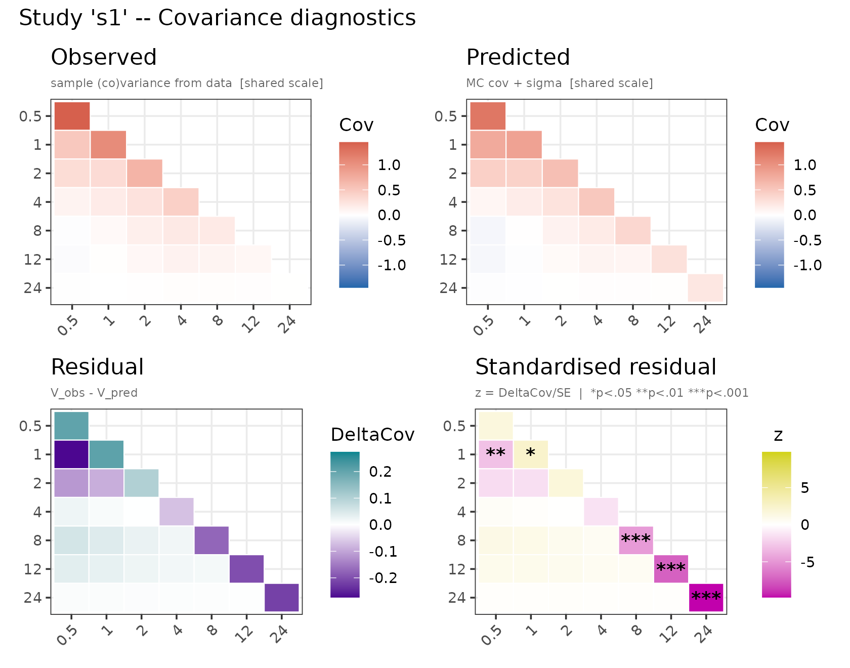

Covariance diagnostics for the additive fit. In the lower-right panel, cells marked with an asterisk are where the predicted covariance differs from the observed by more than the sampling noise in V.

When the residual model fits, the standardised panel looks like noise. Here the diagonal is starred early and late in opposite directions: one constant variance spread over the whole profile, too small where concentrations are high and too large where they have decayed. That opposite-sign pattern is the signature of an additive model on proportional data, and the fix is to refit with prop() or add() + prop().

This panel is the aggregate-data replacement for a residual-vs-predicted plot; see Diagnostic plots.

What you can write

You write the error model in ordinary nlmixr2 syntax; admixr2 adds nothing to the language. The estimator is the constraint: adirmc supports the closed-form continuous models only, because it computes its mean by importance-reweighting samples inside a single compiled routine that knows only those variance forms. admc, adfo and adgh support all of it.

Written as	Estimators	Notes
Continuous — exact, closed form
`cp ~ add(a)`	all four
`cp ~ prop(b)`	all four
`cp ~ pow(b, c)`	all four	exact at `c = 0.5` and `1`; otherwise the moments use a second-order expansion. `c` is an exponent, not an SD
`cp ~ add(a) + prop(b)`	all four	variance `a² + (b·f)²`
`cp ~ add(a) + prop(b) + combined1()`	all four	variance `(a + b·f)²` — a different model, not a reparameterisation of the row above
`cp ~ lnorm(a)`	all four	moment-matched log-normal
any of the above `+ t(nu)`	all four	fix `nu`: only `a²·nu/(nu−2)` is identified, so a free `nu` returns its starting value
Transformed — integrated numerically
`cp ~ boxCox(lambda) + add(a)`	not `adirmc`	`lambda` estimated or fixed
`cp ~ yeoJohnson(lambda) + add(a)`	not `adirmc`	`lambda` estimated or fixed
`cp ~ logitNorm(a, lo, hi)`	not `adirmc`	for an endpoint with a floor and a ceiling
`cp ~ probitNorm(a, lo, hi)`	not `adirmc`	as above
Discrete — no residual parameters
`y ~ pois(cp)`	not `adirmc`	the prediction is the argument, not the left-hand side
`y ~ binom(N, pp)`	not `adirmc`	`N` is the binomial denominator per observation, not the study’s `n`, and must be constant
`y ~ nbinomMu(k, cp)`	not `adirmc`
`cp ~ c(p1, p2, ...)`	not `adirmc`	ordinal; `p1, p2, ...` are the category probabilities, one observation block each
`y ~ beta(shape1, shape2)`	`admc`, `adgh`	the precision is implied by the two shapes, which `adfo` and `adirmc` cannot reach
Correlated residuals
`cp ~ add(a) + ar(rho)`	not `adirmc`	needs a full observed `V`, and pairs with `add()` only

Each endpoint carries its own error model, so a multi-output model keeps them separate — see Several observed compartments.

nu and rho are the two parameters aggregate data does not identify, and they fail differently. nu enters only through the variance multiplier, so it is aliased with the scale: admixr2 warns and returns your starting value, which is why you should fix it. rho lives in the off-diagonal, so a diagonal V carries no information about it at all, and that is a hard error rather than a warning.

Anything else is refused: lnorm mixed with prop/pow/ar/t, ar with a prediction-dependent variance or a transform, t() with no scale term, cauchy(), and the distributions with no admixr2 implementation. In each case the combination has no single well-defined aggregate mean and variance, so admixr2 refuses rather than fitting something else:

bad <- mod_prop |> model(cp ~ lnorm(res.sd) + prop(b)) |> ini(b = 0.2)

nlmixr2(bad, admData(), est = "adgh", control = adghControl(studies = gen))
#> Error:
#> ! Unsupported residual error model for endpoint 'cp': lnorm() combined with a proportional or power term.
#> 
#>   Why: lnorm()'s parameter is the SD on the LOG scale, which already makes
#>   the residual proportional to the prediction; adding prop()/pow() on top
#>   has no single well-defined aggregate variance.
#> 
#>   admixr2 fits AGGREGATE data -- each study contributes a mean and a
#>   covariance, scored as a multivariate normal -- so the residual model must
#>   reduce to a mean and a variance on the natural scale.
#> 
#>   Fix: Use lnorm(a) alone, or add(a) + prop(b) on the natural scale.
#> 
#> Supported residual error models (f = the model prediction):
#>   add(a)              var = a^2
#>   prop(b)             var = (b*f)^2
#>   pow(b, c)           var = (b*f^c)^2
#>   lnorm(a)            lognormal, moment-matched
#>   add(a) + prop(b)    var = a^2 + (b*f)^2   [combined2, the default]
#>                       var = (a + b*f)^2     [combined1, via combined1()]
#>   add(a) + pow(b, c)  either combined form
#>   ... + t(nu)         any of the above with Student-t residuals (nu > 2):
#>                       the scale family, var = <above> * nu/(nu-2)
#> 
#>   Note: earlier versions of admixr2 accepted this model with a warning and
#>   then fitted it as ADDITIVE error. Any results carried over from that are
#>   not the model you specified.

Setting `resid_nodes` on a transformed endpoint

Writing cp ~ boxCox(lambda) + add(a) says the residual is normal on the transformed scale, not in mg/L. But the study you are fitting reports its mean and SD in mg/L. So admixr2 has to answer a question that never comes up in an individual-level fit: if the residual is normal after transformation, what are the mean and variance back on the original scale?

For add() and prop() that back-transformation has a formula. For boxCox, yeoJohnson, logitNorm and probitNorm it does not. Because the transform bends the residual, the mean of the back-transformed values is not the back-transform of the mean, and there is no closed form for either moment.

admixr2 integrates over the residual instead. This is the same machinery as the Gaussian quadrature used to integrate over the etas in a mixed-effects likelihood — nlmixr2’s agq, or nAGQ in lme4 — aimed at a different integral: over the residual at one observation, rather than over a subject’s random effects.

Concretely: rather than one prediction, the endpoint is evaluated at resid_nodes different residual values, each weighted by how probable it is under the normal, and the results averaged. Two things separate this from simulating residuals.

The values are chosen, not drawn. Gauss-Hermite places n points so that the weighted average is exact whenever the quantity being averaged behaves like a polynomial of degree 2n - 1 or less. A few well-placed points therefore do the work of a great many random draws. They sit symmetrically about zero and reach out to about ±sqrt(2n) residual SDs, so a higher count both resolves the middle and reaches further into the tails.

The grid never moves. The same points at every likelihood evaluation, so the objective is smooth and its gradient usable. Drawing fresh residuals would add Monte Carlo noise to every evaluation, which the optimiser would have to work through.

How many nodes you need depends on how curved the back-transformation is over the range the residual explores. A residual that is narrow on the transformed scale stays where that curve is nearly straight, and a handful of nodes covers it.

The demanding case is a wide residual on a bounded endpoint — logitNorm or probitNorm on a score with a floor and a ceiling — because the back-transform flattens against both bounds. For a logit-normal endpoint with an SD of 2 on the transformed scale, 7 nodes puts the 24 h variance 7% low and 15 nodes 0.6% low; 31 is converged. A more typical residual width converges by about 15. The default of 81 covers the awkward cases with room to spare, at a cost invisible next to the ODE solve. Lower it only if profiling shows the quadrature is your bottleneck, and check that the objective does not move when you do.

resid_nodes is on all four estimator controls and on datagenControl(), so a study you generate and the fit that consumes it integrate the residual the same way unless you change one of them.

How to choose

There is no residual plot to look at. The choice comes from the published error bars, from what the source papers already report, and from the diagnostics above.

Read the error bars. Widening roughly in proportion to the mean points to prop(); roughly constant width across the profile points to add(); wide at the top and not shrinking to nothing at the bottom points to add() + prop().
Take the residual from the source where one is reported. A study that published its own population model has already estimated a residual error model from the individual data you do not have — better information than an aggregate fit can recover. Supply that model to datagen() and it comes along with it, or carry it across by fixing yours to the same value:
```
ini({ res.sd <- fix(0.15) })   # residual error reported by the source study
```
Ask whether one residual across studies is credible. Studies run in different laboratories, on different assays, years apart will not share a residual magnitude. A single pooled residual is an assumption, not a default. If one study’s error bars are much wider relative to its means than the rest, give that study’s endpoint its own residual rather than letting it set the value for every study.
Bounded endpoints belong on a transformed scale. A score with a floor and a ceiling should use logitNorm() or probitNorm(), not add(), which will happily predict outside the range without warning.
Then check. Fit the candidates, compare objectives, and read the covariance panel. A residual model that fits leaves no structure in the standardised residual.

The residual and the IIV are separated only by their different time-course. This is the constraint behind everything above. Where the two have a similar shape — a proportional residual against IIV on a parameter that scales the whole profile — they trade off, and the split is weakly determined. The worked example is that failure in miniature: the misspecified residual put its missing variance straight into omega.v.

This is also an argument for the thing admixr2 is for. One study with few time points barely identifies the split. Several studies at different doses and sampling schedules constrain it from more directions at once, which is why a meta-analysis across studies is better posed here than a reanalysis of any one of them.

How the residual enters the covariance

This is the one place where admixr2 changed behaviour in the current release, and the change moves results for most models, so it is worth being precise about.

Both the old and the new rule start from the same structural covariance Cov(f) — the spread caused by subjects differing from one another — and then account for the residual on top of it. They differ in what they add.

Up to version 0.3.0, the residual variance was worked out once, at the population mean prediction, and added to the diagonal:

$V \;=\; \mathrm{Cov}(f) \;+\; \mathrm{diag}\big(\Sigma(\bar f)\big), \qquad \text{proportional: } \Sigma(\bar f) \;=\; b^2\,\bar f^{\,2}$

This is the “no eta-eps interaction” convention, familiar from individual-level fitting, where each observation has its own prediction and the question does not arise.

From this release, the residual variance is averaged over subjects — the law of total variance:

$V \;=\; \mathrm{Cov}(f) \;+\; \mathrm{diag}\big(\mathbb{E}_\eta[\mathrm{Var}(y \mid \eta)]\big), \qquad \text{proportional: } b^2\,\mathbb{E}[f^2] \;=\; b^2\big(\bar f^{\,2} + \mathrm{Var}(f)\big)$

The two differ by exactly b^2 Var(f). A subject’s residual scales with that subject’s prediction, not with the population mean, and the average of a square exceeds the square of the average by the between-subject variance. The old rule drops that term.

error model	up to 0.3.0 added	now adds
`add(a)`	`a²`	`a²` — unchanged
`prop(b)`	`b²·mean²`	`b²·(mean² + Var(f))`
`pow(b, c)`	`b²·mean^(2c)`	`b²·E[f^(2c)]`
`lnorm(a)`	the diagonal only	the diagonal, and the off-diagonals scaled by `exp(s)`

lnorm() is the one that is not only a diagonal correction: its conditional mean is f·exp(s/2), so the whole covariance is scaled, not just its diagonal.

Against the simulated subjects from earlier, where the residual’s true contribution is known:

Open circles are the residual variance measured from the simulated subjects. Averaging over subjects lands on them; evaluating at the population mean drifts low as subjects spread apart.

The new rule agrees with the measurement to within 0.6% at every time. The old one is fine early, where subjects are alike, and misses 74% of the residual by 24 h, where they differ from one another by more than the mean itself.

What this means for results you already have. Purely additive models are unaffected, bit for bit — a² does not depend on the prediction, so there is nothing to average. Every prop(), pow() and lnorm() fit changes. Checked against individual-level simulation, the old rule carried a fixed 15-20% bias in the predicted variance that did not shrink as the study grew; in a proportional model with 30-50% IIV the reported residual SD and omega were each biased upward by roughly 2-4%, and for lnorm() the effect is larger. A refit will not reproduce the numbers a 0.3.0 fit gave you, and the new ones are the correct comparison to a residual estimated from individual data.

Two caveats

Point estimates are recovered; the reported uncertainty is approximate. The covariance term of the objective treats your observed V as coming from normally distributed subjects. That holds for add/prop/pow/lnorm, and is an approximation for a heavy-tailed or bounded per-subject residual (small-nu t, counts, beta). State it when reporting SEs or intervals from those.
New since 0.3.0. That release supported add, prop, pow, both combined forms and lnorm; everything else above was refused. This release adds t(nu), the four transformed endpoints, the discrete endpoints and ordinal, beta() under admc/adgh, ar(rho) with add(), and resid_nodes. It also changes how the residual is composed into the covariance, so prop(), pow() and lnorm() results move — see the section above. If you have results from a version that accepted a now-refused model with only a warning — pow() above all — treat them as suspect: they were fitted as additive error.